Table of Contents
1 Exploring different doubling tricks for different kinds of regret bounds
1.1 What do we want?
1.2 Dependencies
1.3 Defining the functions \(f\)
1.3.1 Cheating with a “safe” log
1.3.2 Geometric sequences
1.3.3 Exponential sequences
1.3.4 Generic function \(f\)
1.3.5 Some specific case of intermediate sequences
1.4 Defining the sequences and last term
1.4.1 Sequence \(f \mapsto (T_i)_i\)
1.4.2 Last term operator \(T \mapsto L_T\)
1.4.3 Helper for the plot
1.5 Plotting what we want
1.5.1 Plotting the values of the sequences
1.5.2 Plotting the ratio for our upper-bound
1.6 Results
1.6.1 Values of the doubling sequences
1.6.2 Bound in \(R_T \leq \mathcal{O}(\log(T))\)
1.6.3 Bound in \(R_T \leq \mathcal{O}(\sqrt{T})\)
1.6.4 Bound in \(R_T \leq \mathcal{O}(\sqrt{T \log(T)})\)
1.6.5 A last weird bound in \(R_T \leq \mathcal{O}(T^{2/3} \log(T))\) (just to try)
1.7 Conclusions
1.7.1 About geometric sequences
1.7.2 About exponential sequences
1.7.3 About intermediate sequences
Exploring different doubling tricks for different kinds of regret bounds
Author: Lilian Besson and Emilie Kaufmann,
License: MIT License.
Date: 19 September 2018.
What do we want?
This notebooks studies and plot the ratio between a sum like the following
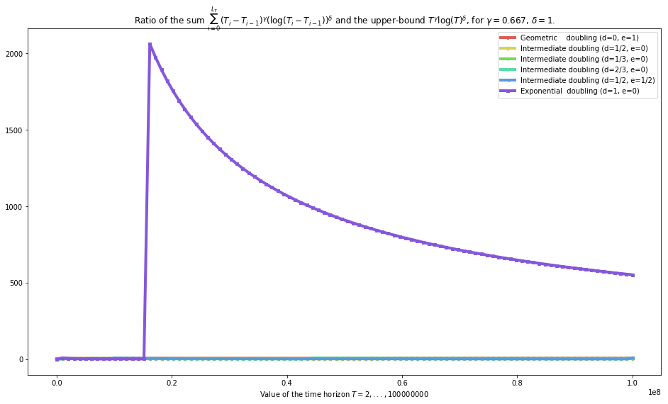
and the quantity \(T^\gamma (\ln(T))^\delta\), where \(T \in\mathbb{N}\) is a time horizon of some multi-armed bandit problem, and \(\gamma,\delta \geq 0\) but not simultaneously zero.
The successive horizon (in a doubling trick scheme) are defined by \(\forall i\in\mathbb{N},\; T_i := \lfloor \exp(\alpha \times \exp(f(i))) \rfloor\), for some function \(f: i \mapsto f(i)\).
We study a generic form of functions \(f\), with parameters \(c,d,e \geq 0\): \(f(i) = c (i^d) (\log(i))^e\).
\(d, e = 0, 1\) corresponds to the geometric doubling trick, with \(T_i = \mathcal{O}(2^i)\),
\(d, e = 1, 0\) corresponds to the exponential doubling trick, with \(T_i = \mathcal{O}(2^{2^i})\),
we are curious about intermediate sequences, that grow faster than any geometric scheme but slower than any exponential scheme. Mathematically, it corresponds to the generic case of \(0 < d < 1\) and \(e \geq 0\).
Moreover, we are especially interested in these two cases: - \(\gamma, \delta = 0, 1\) for bounds in regret like \(R_T(\mathcal{A}) = \mathcal{O}(\log T)\) (stochastic problem and problem dependent bounds), - \(\gamma, \delta = 1/2, 0\) for bounds in regret like \(R_T(\mathcal{A}) = \mathcal{O}(\sqrt{T})\) (stochastic problem and worst-case bounds, ie “minimax bounds”, or adversarial regret).
To conclude these quick explanation, the notation \(L_T\) is the “last term operator”, for a fixed increasing sequence \((T_i)_{i\in\mathbb{N})\):
Dependencies
Here we import some code.
[1]:
!pip install watermark
%load_ext watermark
%watermark -v -m -p numpy,matplotlib,seaborn -a "Lilian Besson and Emilie Kaufmann"
Requirement already satisfied: watermark in ./venv3/lib/python3.6/site-packages (1.7.0)
Requirement already satisfied: ipython in ./venv3/lib/python3.6/site-packages (from watermark) (7.1.1)
Requirement already satisfied: pexpect; sys_platform != "win32" in ./venv3/lib/python3.6/site-packages (from ipython->watermark) (4.6.0)
Requirement already satisfied: prompt-toolkit<2.1.0,>=2.0.0 in ./venv3/lib/python3.6/site-packages (from ipython->watermark) (2.0.7)
Requirement already satisfied: setuptools>=18.5 in ./venv3/lib/python3.6/site-packages (from ipython->watermark) (40.6.2)
Requirement already satisfied: pygments in ./venv3/lib/python3.6/site-packages (from ipython->watermark) (2.2.0)
Requirement already satisfied: pickleshare in ./venv3/lib/python3.6/site-packages (from ipython->watermark) (0.7.5)
Requirement already satisfied: decorator in ./venv3/lib/python3.6/site-packages (from ipython->watermark) (4.3.0)
Requirement already satisfied: jedi>=0.10 in ./venv3/lib/python3.6/site-packages (from ipython->watermark) (0.13.1)
Requirement already satisfied: traitlets>=4.2 in ./venv3/lib/python3.6/site-packages (from ipython->watermark) (4.3.2)
Requirement already satisfied: backcall in ./venv3/lib/python3.6/site-packages (from ipython->watermark) (0.1.0)
Requirement already satisfied: ptyprocess>=0.5 in ./venv3/lib/python3.6/site-packages (from pexpect; sys_platform != "win32"->ipython->watermark) (0.6.0)
Requirement already satisfied: six>=1.9.0 in ./venv3/lib/python3.6/site-packages (from prompt-toolkit<2.1.0,>=2.0.0->ipython->watermark) (1.11.0)
Requirement already satisfied: wcwidth in ./venv3/lib/python3.6/site-packages (from prompt-toolkit<2.1.0,>=2.0.0->ipython->watermark) (0.1.7)
Requirement already satisfied: parso>=0.3.0 in ./venv3/lib/python3.6/site-packages (from jedi>=0.10->ipython->watermark) (0.3.1)
Requirement already satisfied: ipython-genutils in ./venv3/lib/python3.6/site-packages (from traitlets>=4.2->ipython->watermark) (0.2.0)
Lilian Besson and Emilie Kaufmann

CPython 3.6.6
IPython 7.1.1

numpy 1.15.4
matplotlib 3.0.2
seaborn 0.9.0

compiler   : GCC 8.0.1 20180414 (experimental) [trunk revision 259383
system     : Linux
release    : 4.15.0-38-generic
machine    : x86_64
processor  : x86_64
CPU cores  : 4
interpreter: 64bit
[3]:
from __future__ import division, print_function  # Python 2 compatibility

__author__ = "Lilian Besson and Emilie Kaufmann"

import numpy as np
import matplotlib as mpl
import matplotlib.pyplot as plt
import seaborn as sns
[4]:
mpl.rcParams['figure.figsize'] = (16, 9)
Change here if needed, use 128 bits floats instead of 64 bits.
[5]:
_f = np.float
_f = np.float128
Defining the functions \(f\)
Let’s start by defining the functions.
This is some experimental code to plot some doubling sequences and check numerically some inequalities : like controlling a sum \(\Sigma_i=0^n u_i\) by a constant times to last term \(u_n\) and controlling the last term \(u_{L_T}\) as a function of \(T\).
[6]:
#: The constant c in front of the function f.
constant_c_for_the_functions_f = _f(1.0)
constant_c_for_the_functions_f = _f(0.1)
constant_c_for_the_functions_f = _f(0.5)
We recall that we are interested by sequences \((T_i)_i\) that grows about
and
for \(c > 0, d \geq 0, e \geq 0\) and \(d, e\) not zero simultaneously.
Cheating with a “safe” log
I don’t want to have \(\log(T_i - T_{i-1}) = -\infty\) if \(T_i = T_{i-1}\) but I want \(\log(0) = 0\). Let’s hack it!
[7]:
def mylog(x):
    res = np.log(x)
    if np.shape(res):
        res[np.isinf(res)] = _f(0.0)
    else:
        if np.isinf(res):
            res = _f(0.0)
    return res
Geometric sequences
[8]:
def function_f__for_geometric_sequences(i, c=constant_c_for_the_functions_f):
    r""" For the *geometric* doubling sequences, :math:`f(i) = c \times \log(i)`."""
    if i <= 0: return _f(0.0)
    return c * mylog(i)
Exponential sequences
[9]:
def function_f__for_exponential_sequences(i, c=constant_c_for_the_functions_f):
    r""" For the *exponential* doubling sequences, :math:`f(i) = c \times i`."""
    return c * i
Generic function \(f\)
As soon as \(0 < d < 1\), no matter the value of \(e\), \(T_i\) will essentially faster than any geometric sequence and slower than any exponential sequence.
[10]:
def function_f__for_generic_sequences(i, c=constant_c_for_the_functions_f, d=_f(0.5), e=_f(0.0)):
    r""" For a certain *generic* family of doubling sequences, :math:`f(i) = c \times i^{d} \times (\log(i))^{e}`.

    - ``d, e = 0, 1`` gives :func:`function_f__for_geometric_sequences`,
    - ``d, e = 1, 0`` gives :func:`function_f__for_geometric_sequences`,
    - ``d, e = 0.5, 0`` gives an intermediate sequence, growing faster than any geometric sequence and slower than any exponential sequence,
    - any other combination has not been studied yet.

    .. warning:: ``d`` should most probably be smaller than 1.
    """
    i = float(i)
    if i <= 0: return _f(0.0)
    if e == 0:
        assert d > 0, "Error: invalid value of d = {} for function_f__for_generic_sequences, cannot be <= 0.".format(d)  # DEBUG
        return c * (i ** d)
    assert e > 0, "Error: invalid value of e = {} for function_f__for_generic_sequences, cannot be <= 0.".format(e)  # DEBUG
    if d == 0:
        return c * ((mylog(i)) ** e)
    return c * (i ** d) * ((mylog(i)) ** e)
Some specific case of intermediate sequences
Analytically (mathematically) we started to study \(f(i) = \sqrt{i}\).
[11]:
def function_f__for_intermediate_sequences(i):
    return function_f__for_generic_sequences(i, c=constant_c_for_the_functions_f, d=_f(0.5), e=_f(0.0))
And empirically, I’m curious about other sequences, including \(f(i) = i^{1/3}\), \(f(i) = i^{2/3}\) and \(f(i) = \sqrt{i} \sqrt{\log(i)}\).
[12]:
def function_f__for_intermediate2_sequences(i):
    return function_f__for_generic_sequences(i, c=constant_c_for_the_functions_f, d=_f(0.3333), e=_f(0.0))

def function_f__for_intermediate3_sequences(i):
    return function_f__for_generic_sequences(i, c=constant_c_for_the_functions_f, d=_f(0.6667), e=_f(0.0))

def function_f__for_intermediate4_sequences(i):
    return function_f__for_generic_sequences(i, c=constant_c_for_the_functions_f, d=_f(0.5), e=_f(0.5))
Defining the sequences and last term
[13]:
#: Value of the parameter :math:`\alpha` for the :func:`Ti_from_f` function.
alpha_for_Ti = _f(0.1)
alpha_for_Ti = _f(1.0)
alpha_for_Ti = _f(0.5)
Sequence \(f \mapsto (T_i)_i\)
We need to define a function that take \(f\) and give the corresponding sequence \((T_i)\), given as a function \(Ti: i \mapsto T_i\).
[14]:
def Ti_from_f(f, alpha=alpha_for_Ti, *args, **kwargs):
    r""" For any non-negative and increasing function :math:`f: i \mapsto f(i)`, the corresponding sequence is defined by:

    .. math:: \forall i\in\mathbb{N},\; T_i := \lfloor \exp(\alpha \times \exp(f(i))) \rfloor.

    .. warning:: :math:`f(i)` can need other parameters, see the examples above. They can be given as ``*args`` or ``**kwargs`` to :func:`Ti_from_f`.

    .. warning:: it should be computed otherwise, I should give :math:`i \mapsto \exp(f(i))` instead of :math:`f: i \mapsto f(i)`. I need to try as much as possible to reduce the risk of overflow errors!
    """
    # WARNING don't forget the floor!
    def Ti(i):
        this_Ti = np.floor(np.exp(alpha * np.exp(f(float(i), *args, **kwargs))))
        if not (np.isinf(this_Ti) or np.isnan(this_Ti)):
            this_Ti = int(this_Ti)
        # print("    For f = {}, i = {} gives Ti = {}".format(f, i, this_Ti))  # DEBUG
        return this_Ti
    return Ti
Last term operator \(T \mapsto L_T\)
Then we can define the “last term operator”, by a naive search (and not an analytic derivation). I don’t care if this is not efficient, it works and at least we are sure that \(L_T\) satisfies its definition.
[15]:
def last_term_operator_LT(Ti, max_i=10000):
    r""" For a certain function representing a doubling sequence, :math:`T: i \mapsto T_i`, this :func:`last_term_operator_LT` function returns the function :math:`L: T \mapsto L_T`, defined as:

    .. math:: \forall T\in\mathbb{N},\; L_T := \min\{ i \in\mathbb{N},\; T \leq T_i \}.

    :math:`L_T` is the only integer which satisfies :math:`T_{L_T - 1} < T \leq T_{L_T}`.
    """
    def LT(T, max_i=max_i):
        i = 0
        while Ti(i) < T:  # very naive loop!
            i += 1
            if i >= max_i:
                raise ValueError("LT(T={T}) was unable to find a i <= {max_i} such that T_i >= T.".format(T, max_i))  # DEBUG
        assert Ti(i - 1) < T <= Ti(i), "Error: i = {} was computed as LT for T = {} and Ti = {} but does not satisfy T_(i-1) < T <= T(i)".format(i, T, Ti)  # DEBUG
        # print("  For LT: i = {} was computed as LT for T = {} and Ti = {} and satisfies T(i-1) = {} < T <= T(i) = {}".format(i, T, Ti, Ti(i-1), Ti(i)))  # DEBUG
        return i
    return LT
Helper for the plot
[16]:
def markers_colors(nb):
    """Make unique markers and colors for nb plots."""
    allmarkers = ['o', 'D', 'v', 'p', '<', 's', '^', '*', 'h', '>']
    longlist = allmarkers * (1 + int(nb / float(len(allmarkers))))  # Cycle the good number of time
    markers = longlist[:nb]  # Truncate
    colors = sns.hls_palette(nb + 1)[:nb]
    return markers, colors
Plotting what we want
By default, we will study the following doubling sequences:
Geometric doubling with \(d=0, e=1\),
Intermediate doubling with \(d=1/2, e=0\) (the one I’m excited about),
Intermediate doubling with \(d=1/3, e=0\),
Intermediate doubling with \(d=2/3, e=0\),
Intermediate doubling with \(d=1/2, e=1/2\),
Exponential doubling with \(d=1, e=0\).
Plotting the values of the sequences
First, we want to check how much do these sequences increase.
[17]:
def plot_doubling_sequences(
        i_min=1, i_max=30,
        list_of_f=(
            function_f__for_geometric_sequences,
            function_f__for_intermediate_sequences,
            function_f__for_intermediate2_sequences,
            function_f__for_intermediate3_sequences,
            function_f__for_intermediate4_sequences,
            function_f__for_exponential_sequences,
            ),
        label_of_f=(
            "Geometric    doubling (d=0, e=1)",
            "Intermediate doubling (d=1/2, e=0)",
            "Intermediate doubling (d=1/3, e=0)",
            "Intermediate doubling (d=2/3, e=0)",
            "Intermediate doubling (d=1/2, e=1/2)",
            "Exponential  doubling (d=1, e=0)",
            ),
        *args, **kwargs
    ):
    r""" Display a plot to illustrate the values of the :math:`T_i` as a function of :math:`i` for some i.

    - Can accept many functions f (and labels).
    """
    markers, colors = markers_colors(len(list_of_f))
    fig = plt.figure()

    i_s = np.arange(i_min, i_max, dtype=np.float128)
    # now for each function f
    for num_f, (f, la) in enumerate(zip(list_of_f, label_of_f)):
        print("\n\nThe {}th function is referred to as {} and is {}".format(num_f, la, f))  # DEBUG
        Ti = Ti_from_f(f)
        values_of_Ti = [Ti(i) for i in i_s]
        plt.plot(i_s, values_of_Ti, label=la, lw=4, ms=7, color=colors[num_f], marker=markers[num_f])

    plt.legend()
    plt.xlabel(r"Value of the time horizon $i = {},...,{}$".format(i_min, i_max))
    plt.title(r"Comparison of the values of $T_i$")
    plt.show()
    # return fig
Plotting the ratio for our upper-bound
[18]:
def plot_quality_first_upper_bound(
        Tmin=2, Tmax=int(1e8), nbTs=100,
        gamma=_f(0.0), delta=_f(1.0),  # XXX bound in RT <= log(T)
        # gamma=_f(0.5), delta=_f(0.0),  # XXX bound in RT <= sqrt(T)
        # gamma=_f(0.5), delta=_f(0.5),  # XXX bound in RT <= sqrt(T * log(T))
        # gamma=_f(0.66667), delta=_f(1.0),  # XXX another weird bound in RT <= T^2/3 * log(T)
        list_of_f=(
            function_f__for_geometric_sequences,
            function_f__for_intermediate_sequences,
            function_f__for_intermediate2_sequences,
            function_f__for_intermediate3_sequences,
            function_f__for_intermediate4_sequences,
            function_f__for_exponential_sequences,
            ),
        label_of_f=(
            "Geometric    doubling (d=0, e=1)",
            "Intermediate doubling (d=1/2, e=0)",
            "Intermediate doubling (d=1/3, e=0)",
            "Intermediate doubling (d=2/3, e=0)",
            "Intermediate doubling (d=1/2, e=1/2)",
            "Exponential  doubling (d=1, e=0)",
            ),
        show_Ti_m_Tim1=True,
        *args, **kwargs
    ):
    r""" Display a plot to compare numerically between the following sum :math:`S` and the upper-bound we hope to have, :math:`T^{\gamma} (\log T)^{\delta}`, as a function of :math:`T` for some values between :math:`T_{\min}` and :math:`T_{\max}`:

    .. math:: S := \sum_{i=0}^{L_T} (T_i - T_{i-1})^{\gamma} (\log (T_i - T_{i-1}))^{\delta}.

    - Can accept many functions f (and labels).
    - Can use :math:`T_i` instead of :math:`T_i - T_{i-1}` if ``show_Ti_m_Tim1=False`` (default is to use the smaller possible bound, with difference of sequence lengths, :math:`T_i - T_{i-1}`).

    .. warning:: This is still ON GOING WORK.
    """
    markers, colors = markers_colors(len(list_of_f))
    fig = plt.figure()

    Ts = np.floor(np.linspace(_f(Tmin), _f(Tmax), num=nbTs, dtype=np.float128))
    the_bound_we_want = (Ts ** gamma) * (mylog(Ts) ** delta)

    # now for each function f
    for num_f, (f, la) in enumerate(zip(list_of_f, label_of_f)):
        print("\n\nThe {}th function is referred to as {} and is {}".format(num_f, la, f))  # DEBUG
        Ti = Ti_from_f(f)
        LT = last_term_operator_LT(Ti)
        the_sum_we_have = np.zeros_like(Ts, dtype=np.float128)
        for j, Tj in enumerate(Ts):
            LTj = LT(Tj)
            if show_Ti_m_Tim1:
                the_sum_we_have[j] = sum(
                    ((Ti(i)-Ti(i-1)) ** gamma) * (mylog((Ti(i)-Ti(i-1))) ** delta)
                    for i in range(1, LTj + 1)
                )
            else:
                the_sum_we_have[j] = sum(
                    (Ti(i) ** gamma) * (mylog(Ti(i)) ** delta)
                    for i in range(0, LTj + 1)
                )
            # print("For j = {}, Tj = {}, gives LTj = {}, and the value of the sum from i=0 to LTj is = \n{}.".format(j, Tj, LTj, the_sum_we_have[j]))  # DEBUG
        plt.plot(Ts, the_sum_we_have / the_bound_we_want, label=la, lw=4, ms=4, color=colors[num_f], marker=markers[num_f])

    plt.legend()
    plt.xlabel(r"Value of the time horizon $T = {},...,{}$".format(Tmin, Tmax))
    str_of_Tj_or_dTj = "T_i - T_{i-1}" if show_Ti_m_Tim1 else "T_i"
    plt.title(r"Ratio of the sum $\sum_{i=0}^{L_T} (%s)^{\gamma} (\log(%s))^{\delta}$ and the upper-bound $T^{\gamma} \log(T)^{\delta}$, for $\gamma=%.3g$, $\delta=%.3g$." % (str_of_Tj_or_dTj, str_of_Tj_or_dTj, gamma, delta))  # DEBUG
    plt.show()
    # return fig
Results
Values of the doubling sequences
We check that the exponential sequence is growing WAY faster than all the others.
[19]:
plot_doubling_sequences()
The 0th function is referred to as Geometric    doubling (d=0, e=1) and is <function function_f__for_geometric_sequences at 0x7f0e2cbc3ea0>


The 1th function is referred to as Intermediate doubling (d=1/2, e=0) and is <function function_f__for_intermediate_sequences at 0x7f0e2cbd3ae8>


The 2th function is referred to as Intermediate doubling (d=1/3, e=0) and is <function function_f__for_intermediate2_sequences at 0x7f0e2cbd3f28>


The 3th function is referred to as Intermediate doubling (d=2/3, e=0) and is <function function_f__for_intermediate3_sequences at 0x7f0e2cbe0048>


The 4th function is referred to as Intermediate doubling (d=1/2, e=1/2) and is <function function_f__for_intermediate4_sequences at 0x7f0e2cbe00d0>


The 5th function is referred to as Exponential  doubling (d=1, e=0) and is <function function_f__for_exponential_sequences at 0x7f0e2cbd3268>
/home/lilian/ownCloud/owncloud.crans.org/Crans/These_2016-17/src/SMPyBandits/notebooks/venv3/lib/python3.6/site-packages/ipykernel_launcher.py:12: RuntimeWarning: overflow encountered in exp
  if sys.path[0] == '':
---------------------------------------------------------------------------
OverflowError                             Traceback (most recent call last)
<ipython-input-19-d34d7af5c931> in <module>
----> 1 plot_doubling_sequences()

<ipython-input-17-fb497b0fdf32> in plot_doubling_sequences(i_min, i_max, list_of_f, label_of_f, *args, **kwargs)
     32         Ti = Ti_from_f(f)
     33         values_of_Ti = [Ti(i) for i in i_s]
---> 34         plt.plot(i_s, values_of_Ti, label=la, lw=4, ms=7, color=colors[num_f], marker=markers[num_f])
     35
     36     plt.legend()

/tmp/SMPyBandits/notebooks/venv3/lib/python3.6/site-packages/matplotlib/pyplot.py in plot(scalex, scaley, data, *args, **kwargs)
   2811     return gca().plot(
   2812         *args, scalex=scalex, scaley=scaley, **({"data": data} if data
-> 2813         is not None else {}), **kwargs)
   2814
   2815

/tmp/SMPyBandits/notebooks/venv3/lib/python3.6/site-packages/matplotlib/__init__.py in inner(ax, data, *args, **kwargs)
   1808                         "the Matplotlib list!)" % (label_namer, func.__name__),
   1809                         RuntimeWarning, stacklevel=2)
-> 1810             return func(ax, *args, **kwargs)
   1811
   1812         inner.__doc__ = _add_data_doc(inner.__doc__,

/tmp/SMPyBandits/notebooks/venv3/lib/python3.6/site-packages/matplotlib/axes/_axes.py in plot(self, scalex, scaley, *args, **kwargs)
   1610
   1611         for line in self._get_lines(*args, **kwargs):
-> 1612             self.add_line(line)
   1613             lines.append(line)
   1614

/tmp/SMPyBandits/notebooks/venv3/lib/python3.6/site-packages/matplotlib/axes/_base.py in add_line(self, line)
   1893             line.set_clip_path(self.patch)
   1894
-> 1895         self._update_line_limits(line)
   1896         if not line.get_label():
   1897             line.set_label('_line%d' % len(self.lines))

/tmp/SMPyBandits/notebooks/venv3/lib/python3.6/site-packages/matplotlib/axes/_base.py in _update_line_limits(self, line)
   1915         Figures out the data limit of the given line, updating self.dataLim.
   1916         """
-> 1917         path = line.get_path()
   1918         if path.vertices.size == 0:
   1919             return

/tmp/SMPyBandits/notebooks/venv3/lib/python3.6/site-packages/matplotlib/lines.py in get_path(self)
    943         """
    944         if self._invalidy or self._invalidx:
--> 945             self.recache()
    946         return self._path
    947

/tmp/SMPyBandits/notebooks/venv3/lib/python3.6/site-packages/matplotlib/lines.py in recache(self, always)
    643         if always or self._invalidy:
    644             yconv = self.convert_yunits(self._yorig)
--> 645             y = _to_unmasked_float_array(yconv).ravel()
    646         else:
    647             y = self._y

/tmp/SMPyBandits/notebooks/venv3/lib/python3.6/site-packages/matplotlib/cbook/__init__.py in _to_unmasked_float_array(x)
   1363         return np.ma.asarray(x, float).filled(np.nan)
   1364     else:
-> 1365         return np.asarray(x, float)
   1366
   1367

/tmp/SMPyBandits/notebooks/venv3/lib/python3.6/site-packages/numpy/core/numeric.py in asarray(a, dtype, order)
    499
    500     """
--> 501     return array(a, dtype, copy=False, order=order)
    502
    503

OverflowError: int too large to convert to float
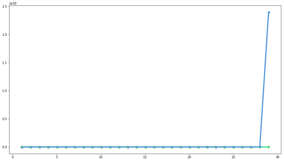
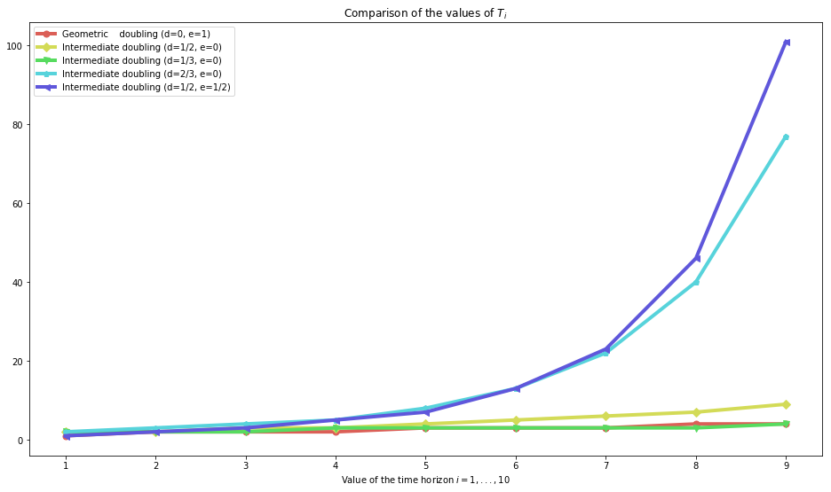
And without this faster sequence, just for the first \(10\) first sequences:
[20]:
plot_doubling_sequences(
    i_max=10,
    list_of_f=(
        function_f__for_geometric_sequences,
        function_f__for_intermediate_sequences,
        function_f__for_intermediate2_sequences,
        function_f__for_intermediate3_sequences,
        function_f__for_intermediate4_sequences,
        ),
    label_of_f=(
        "Geometric    doubling (d=0, e=1)",
        "Intermediate doubling (d=1/2, e=0)",
        "Intermediate doubling (d=1/3, e=0)",
        "Intermediate doubling (d=2/3, e=0)",
        "Intermediate doubling (d=1/2, e=1/2)",
    )
)
The 0th function is referred to as Geometric    doubling (d=0, e=1) and is <function function_f__for_geometric_sequences at 0x7f0e2cbc3ea0>


The 1th function is referred to as Intermediate doubling (d=1/2, e=0) and is <function function_f__for_intermediate_sequences at 0x7f0e2cbd3ae8>


The 2th function is referred to as Intermediate doubling (d=1/3, e=0) and is <function function_f__for_intermediate2_sequences at 0x7f0e2cbd3f28>


The 3th function is referred to as Intermediate doubling (d=2/3, e=0) and is <function function_f__for_intermediate3_sequences at 0x7f0e2cbe0048>


The 4th function is referred to as Intermediate doubling (d=1/2, e=1/2) and is <function function_f__for_intermediate4_sequences at 0x7f0e2cbe00d0>
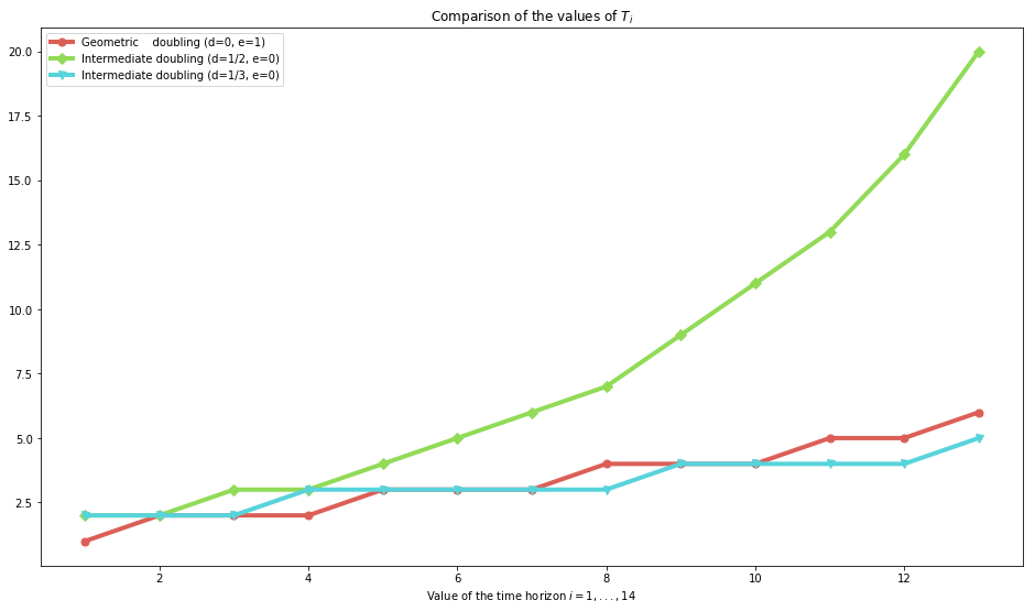
And for the three slower sequences, an interesting observation is that the “intermediate” sequence with \(f(i) = i^{1/3}\) is comparable to \(f(i) = \log(i)\) (geometric one) for small values!
[21]:
plot_doubling_sequences(
    i_max=14,
    list_of_f=(
        function_f__for_geometric_sequences,
        function_f__for_intermediate_sequences,
        function_f__for_intermediate2_sequences,
        ),
    label_of_f=(
        "Geometric    doubling (d=0, e=1)",
        "Intermediate doubling (d=1/2, e=0)",
        "Intermediate doubling (d=1/3, e=0)",
    )
)
The 0th function is referred to as Geometric    doubling (d=0, e=1) and is <function function_f__for_geometric_sequences at 0x7f0e2cbc3ea0>


The 1th function is referred to as Intermediate doubling (d=1/2, e=0) and is <function function_f__for_intermediate_sequences at 0x7f0e2cbd3ae8>


The 2th function is referred to as Intermediate doubling (d=1/3, e=0) and is <function function_f__for_intermediate2_sequences at 0x7f0e2cbd3f28>
Bound in \(R_T \leq \mathcal{O}(\log(T))\)
[22]:
gamma, delta = (_f(0.0), _f(1.0))
[23]:
plot_quality_first_upper_bound(Tmax=int(1e3), gamma=gamma, delta=delta, show_Ti_m_Tim1=True)
The 0th function is referred to as Geometric doubling (d=0, e=1) and is <function function_f__for_geometric_sequences at 0x7f0e2cbc3ea0>
/home/lilian/ownCloud/owncloud.crans.org/Crans/These_2016-17/src/SMPyBandits/notebooks/venv3/lib/python3.6/site-packages/ipykernel_launcher.py:2: RuntimeWarning: divide by zero encountered in log
The 1th function is referred to as Intermediate doubling (d=1/2, e=0) and is <function function_f__for_intermediate_sequences at 0x7f0e2cbd3ae8>


The 2th function is referred to as Intermediate doubling (d=1/3, e=0) and is <function function_f__for_intermediate2_sequences at 0x7f0e2cbd3f28>


The 3th function is referred to as Intermediate doubling (d=2/3, e=0) and is <function function_f__for_intermediate3_sequences at 0x7f0e2cbe0048>


The 4th function is referred to as Intermediate doubling (d=1/2, e=1/2) and is <function function_f__for_intermediate4_sequences at 0x7f0e2cbe00d0>


The 5th function is referred to as Exponential  doubling (d=1, e=0) and is <function function_f__for_exponential_sequences at 0x7f0e2cbd3268>
[24]:
plot_quality_first_upper_bound(gamma=gamma, delta=delta, show_Ti_m_Tim1=False)
The 0th function is referred to as Geometric    doubling (d=0, e=1) and is <function function_f__for_geometric_sequences at 0x7f0e2cbc3ea0>


The 1th function is referred to as Intermediate doubling (d=1/2, e=0) and is <function function_f__for_intermediate_sequences at 0x7f0e2cbd3ae8>


The 2th function is referred to as Intermediate doubling (d=1/3, e=0) and is <function function_f__for_intermediate2_sequences at 0x7f0e2cbd3f28>


The 3th function is referred to as Intermediate doubling (d=2/3, e=0) and is <function function_f__for_intermediate3_sequences at 0x7f0e2cbe0048>


The 4th function is referred to as Intermediate doubling (d=1/2, e=1/2) and is <function function_f__for_intermediate4_sequences at 0x7f0e2cbe00d0>


The 5th function is referred to as Exponential  doubling (d=1, e=0) and is <function function_f__for_exponential_sequences at 0x7f0e2cbd3268>
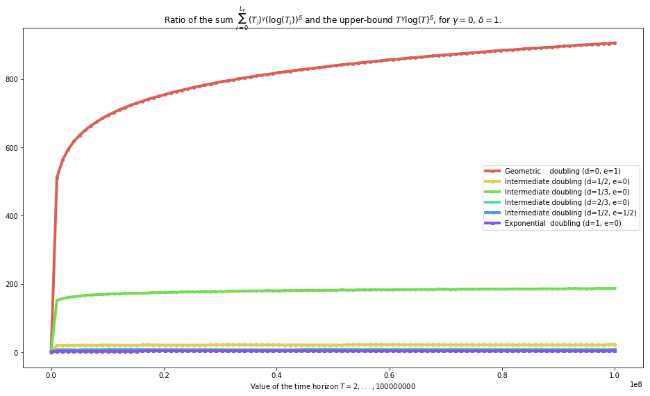
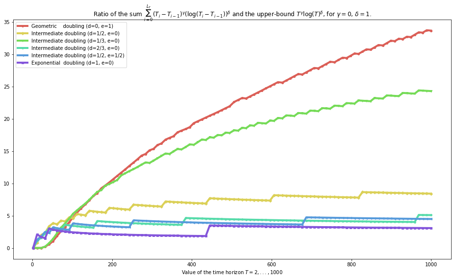
Conclusion: - geometric sequences cannot be used to conserve a logarithmic regret bound (as we proved), - exponential sequences can be used to conserve such bounds (as we proved, also), - and we conjecture that all other sequences (ie as soon as \(d > 0\) ie \(f(i) >> \log(i)\)) can be used too.
Bound in \(R_T \leq \mathcal{O}(\sqrt{T})\)
[25]:
gamma, delta = (_f(0.5), _f(0.0))
[26]:
plot_quality_first_upper_bound(gamma=gamma, delta=delta, show_Ti_m_Tim1=True)
The 0th function is referred to as Geometric doubling (d=0, e=1) and is <function function_f__for_geometric_sequences at 0x7f0e2cbc3ea0>
/home/lilian/ownCloud/owncloud.crans.org/Crans/These_2016-17/src/SMPyBandits/notebooks/venv3/lib/python3.6/site-packages/ipykernel_launcher.py:2: RuntimeWarning: divide by zero encountered in log
The 1th function is referred to as Intermediate doubling (d=1/2, e=0) and is <function function_f__for_intermediate_sequences at 0x7f0e2cbd3ae8>


The 2th function is referred to as Intermediate doubling (d=1/3, e=0) and is <function function_f__for_intermediate2_sequences at 0x7f0e2cbd3f28>


The 3th function is referred to as Intermediate doubling (d=2/3, e=0) and is <function function_f__for_intermediate3_sequences at 0x7f0e2cbe0048>


The 4th function is referred to as Intermediate doubling (d=1/2, e=1/2) and is <function function_f__for_intermediate4_sequences at 0x7f0e2cbe00d0>


The 5th function is referred to as Exponential  doubling (d=1, e=0) and is <function function_f__for_exponential_sequences at 0x7f0e2cbd3268>
[27]:
plot_quality_first_upper_bound(gamma=gamma, delta=delta, show_Ti_m_Tim1=False)
The 0th function is referred to as Geometric    doubling (d=0, e=1) and is <function function_f__for_geometric_sequences at 0x7f0e2cbc3ea0>


The 1th function is referred to as Intermediate doubling (d=1/2, e=0) and is <function function_f__for_intermediate_sequences at 0x7f0e2cbd3ae8>


The 2th function is referred to as Intermediate doubling (d=1/3, e=0) and is <function function_f__for_intermediate2_sequences at 0x7f0e2cbd3f28>


The 3th function is referred to as Intermediate doubling (d=2/3, e=0) and is <function function_f__for_intermediate3_sequences at 0x7f0e2cbe0048>


The 4th function is referred to as Intermediate doubling (d=1/2, e=1/2) and is <function function_f__for_intermediate4_sequences at 0x7f0e2cbe00d0>


The 5th function is referred to as Exponential  doubling (d=1, e=0) and is <function function_f__for_exponential_sequences at 0x7f0e2cbd3268>
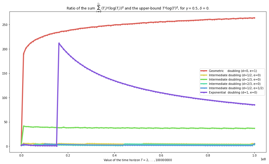
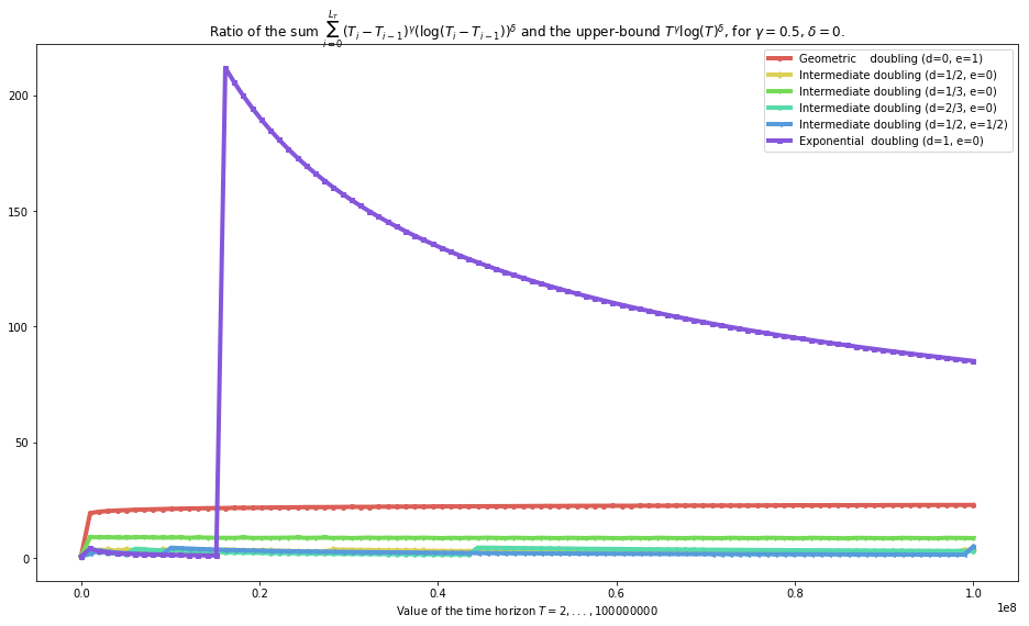
Conclusion: - geometric sequences can be used to conserve a minimax (worst case) regret bound in \(R_T = \mathcal{O}(\sqrt{T})\) (as we proved). > But the proof has to be careful and use a smart bound on \(T_i - T_{i-1} \leq \text{cste} \times b^{i-1}\) and not with a \(b^i\) (see difference between first and second plot) - exponential sequences can be used to conserve such bounds (as we conjectured but did not proved, also), - and we conjecture that all other sequences (ie as soon as \(d > 0\) ie \(f(i) >> \log(i)\)) can be used.
Bound in \(R_T \leq \mathcal{O}(\sqrt{T \log(T)})\)
[28]:
gamma, delta = (_f(0.5), _f(0.5))
[29]:
plot_quality_first_upper_bound(gamma=gamma, delta=delta, show_Ti_m_Tim1=True)
The 0th function is referred to as Geometric doubling (d=0, e=1) and is <function function_f__for_geometric_sequences at 0x7f0e2cbc3ea0>
/home/lilian/ownCloud/owncloud.crans.org/Crans/These_2016-17/src/SMPyBandits/notebooks/venv3/lib/python3.6/site-packages/ipykernel_launcher.py:2: RuntimeWarning: divide by zero encountered in log
The 1th function is referred to as Intermediate doubling (d=1/2, e=0) and is <function function_f__for_intermediate_sequences at 0x7f0e2cbd3ae8>


The 2th function is referred to as Intermediate doubling (d=1/3, e=0) and is <function function_f__for_intermediate2_sequences at 0x7f0e2cbd3f28>


The 3th function is referred to as Intermediate doubling (d=2/3, e=0) and is <function function_f__for_intermediate3_sequences at 0x7f0e2cbe0048>


The 4th function is referred to as Intermediate doubling (d=1/2, e=1/2) and is <function function_f__for_intermediate4_sequences at 0x7f0e2cbe00d0>


The 5th function is referred to as Exponential  doubling (d=1, e=0) and is <function function_f__for_exponential_sequences at 0x7f0e2cbd3268>
[30]:
plot_quality_first_upper_bound(gamma=gamma, delta=delta, show_Ti_m_Tim1=False)
The 0th function is referred to as Geometric    doubling (d=0, e=1) and is <function function_f__for_geometric_sequences at 0x7f0e2cbc3ea0>


The 1th function is referred to as Intermediate doubling (d=1/2, e=0) and is <function function_f__for_intermediate_sequences at 0x7f0e2cbd3ae8>


The 2th function is referred to as Intermediate doubling (d=1/3, e=0) and is <function function_f__for_intermediate2_sequences at 0x7f0e2cbd3f28>


The 3th function is referred to as Intermediate doubling (d=2/3, e=0) and is <function function_f__for_intermediate3_sequences at 0x7f0e2cbe0048>


The 4th function is referred to as Intermediate doubling (d=1/2, e=1/2) and is <function function_f__for_intermediate4_sequences at 0x7f0e2cbe00d0>


The 5th function is referred to as Exponential  doubling (d=1, e=0) and is <function function_f__for_exponential_sequences at 0x7f0e2cbd3268>
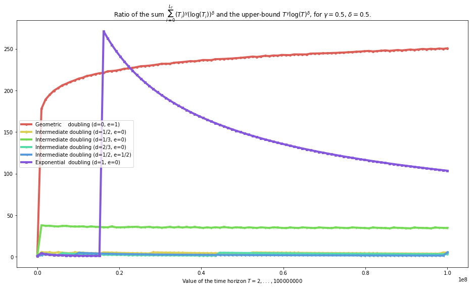
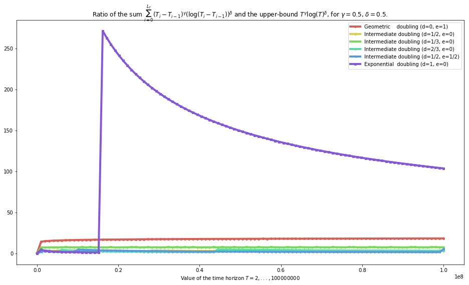
Conclusion: - geometric sequences can be used to conserve a minimax (worst case) regret bound in \(R_T = \mathcal{O}(\sqrt{T \log(T)})\) (as we proved). > But the proof has to be careful and use a smart bound on \(T_i - T_{i-1} \leq \text{cste} \times b^{i-1}\) and not with a \(b^i\) (see difference between first and second plot) - exponential sequences can be used to conserve such bounds (as we conjectured but did not proved, also), - and we conjecture that all other sequences (ie as soon as \(d > 0\) ie \(f(i) >> \log(i)\)) can be used.
A last weird bound in \(R_T \leq \mathcal{O}(T^{2/3} \log(T))\) (just to try)
[31]:
gamma, delta = (_f(0.66667), _f(1.0))
[32]:
plot_quality_first_upper_bound(gamma=gamma, delta=delta, show_Ti_m_Tim1=True)
The 0th function is referred to as Geometric doubling (d=0, e=1) and is <function function_f__for_geometric_sequences at 0x7f0e2cbc3ea0>
/home/lilian/ownCloud/owncloud.crans.org/Crans/These_2016-17/src/SMPyBandits/notebooks/venv3/lib/python3.6/site-packages/ipykernel_launcher.py:2: RuntimeWarning: divide by zero encountered in log
The 1th function is referred to as Intermediate doubling (d=1/2, e=0) and is <function function_f__for_intermediate_sequences at 0x7f0e2cbd3ae8>


The 2th function is referred to as Intermediate doubling (d=1/3, e=0) and is <function function_f__for_intermediate2_sequences at 0x7f0e2cbd3f28>


The 3th function is referred to as Intermediate doubling (d=2/3, e=0) and is <function function_f__for_intermediate3_sequences at 0x7f0e2cbe0048>


The 4th function is referred to as Intermediate doubling (d=1/2, e=1/2) and is <function function_f__for_intermediate4_sequences at 0x7f0e2cbe00d0>


The 5th function is referred to as Exponential  doubling (d=1, e=0) and is <function function_f__for_exponential_sequences at 0x7f0e2cbd3268>
[33]:
plot_quality_first_upper_bound(gamma=gamma, delta=delta, show_Ti_m_Tim1=False)
The 0th function is referred to as Geometric    doubling (d=0, e=1) and is <function function_f__for_geometric_sequences at 0x7f0e2cbc3ea0>


The 1th function is referred to as Intermediate doubling (d=1/2, e=0) and is <function function_f__for_intermediate_sequences at 0x7f0e2cbd3ae8>


The 2th function is referred to as Intermediate doubling (d=1/3, e=0) and is <function function_f__for_intermediate2_sequences at 0x7f0e2cbd3f28>


The 3th function is referred to as Intermediate doubling (d=2/3, e=0) and is <function function_f__for_intermediate3_sequences at 0x7f0e2cbe0048>


The 4th function is referred to as Intermediate doubling (d=1/2, e=1/2) and is <function function_f__for_intermediate4_sequences at 0x7f0e2cbe00d0>


The 5th function is referred to as Exponential  doubling (d=1, e=0) and is <function function_f__for_exponential_sequences at 0x7f0e2cbd3268>
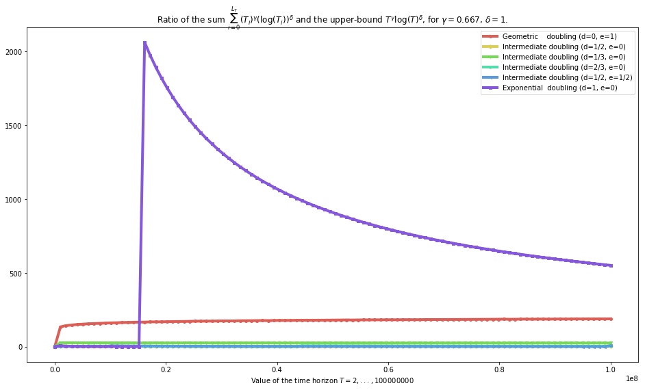
Conclusion: - geometric sequences can be used to conserve a minimax (worst case) regret bound in \(R_T = \mathcal{O}(T^{\gamma} (\log(T))^{\delta})\) (as we proved in the generic case) > But the proof has to be careful and use a smart bound on \(T_i - T_{i-1} \leq \text{cste} \times b^{i-1}\) and not with a \(b^i\) (see difference between first and second plot) - exponential sequences can be used to conserve such bounds (as we conjectured but did not proved, also), - and we conjecture that all other sequences (ie as soon as \(d > 0\) ie \(f(i) >> \log(i)\)) can be used.
Conclusions
The take home messages are the following:
About geometric sequences
We can see that bounding \(T_i - T_{i-1}\) by \(T_i\) usually is strongly sub-optimal for the geometric sequences, as we saw it in our paper, but works fine for the other sequences.
We could check that (numerically) a geometric sequence grows too slowly to preserve a logarithmic bound \(R_T \leq \mathcal{O}(\log(T))\) (first plot), as we proved.
About exponential sequences
They work perfectly fine to preserve logarithmic regret bound, as we proved.
And as we conjectured, they (seem to) work perfectly fine too to preserve minimax (worst case) regret bound, even if we failed to prove it completely so far.
About intermediate sequences
They (seem to) work perfectly fine to preserve logarithmic regret bound, as we started to prove it (work in progress).
And as we conjectured, they (seem to) work perfectly fine too to preserve minimax (worst case) regret bound, as we started to prove it (work in progress).
That’s it for today!