Table of Contents¶

1 Trying to use Black-Box Bayesian optimization algorithms for a Gaussian bandit problem

1.1 Creating the Gaussian bandit problem

1.2 Using a Black-Box optimization algorithm

1.2.1 Implementation

1.3 Comparing its performance on this Gaussian problem

1.3.1 Configuring an experiment

1.3.2 Running an experiment

1.3.3 Visualizing the results

1.4 Another experiment, with just more Gaussian arms

1.4.1 Running the experiment

1.4.2 Visualizing the results

1.4.3 Very good performance!

1.5 Another experiment, with Bernoulli arms

1.5.1 Running the experiment

1.5.2 Visualizing the results

1.5.3 Very good performances also!

1.6 Conclusion

1.6.1 Non-logarithmic regret ?

1.6.2 Comparing time complexity

Trying to use Black-Box Bayesian optimization algorithms for a Gaussian bandit problem¶

This small Jupyter notebook presents an experiment, in the context of Multi-Armed Bandit problems (MAB).

I am trying to answer a simple question:

“Can we use generic black-box Bayesian optimization algorithm, like a Gaussian process or Bayesian random forest, instead of MAB algorithms like UCB or Thompson Sampling ?

I will use my SMPyBandits library, for which a complete documentation is available, here at https://smpybandits.github.io/, and the scikit-optimize package (skopt).

Creating the Gaussian bandit problem¶

First, be sure to be in the main folder, or to have installed `SMPyBandits <https://github.com/SMPyBandits/SMPyBandits>`__, and import the `MAB class <https://smpybandits.github.io/docs/Environment.MAB.html#Environment.MAB.MAB>`__ from the ``Environment` package <https://smpybandits.github.io/docs/Environment.html#module-Environment>`__:

[2]:

import numpy as np

[3]:

!pip install SMPyBandits watermark
%load_ext watermark
%watermark -v -m -p SMPyBandits -a "Lilian Besson"

Requirement already satisfied: SMPyBandits in ./venv3/lib/python3.6/site-packages (0.9.4)
Requirement already satisfied: watermark in ./venv3/lib/python3.6/site-packages (1.7.0)
Requirement already satisfied: scikit-learn in ./venv3/lib/python3.6/site-packages (from SMPyBandits) (0.20.0)
Requirement already satisfied: numpy in ./venv3/lib/python3.6/site-packages (from SMPyBandits) (1.15.4)
Requirement already satisfied: scikit-optimize in ./venv3/lib/python3.6/site-packages (from SMPyBandits) (0.5.2)
Requirement already satisfied: seaborn in ./venv3/lib/python3.6/site-packages (from SMPyBandits) (0.9.0)
Requirement already satisfied: scipy>0.9 in ./venv3/lib/python3.6/site-packages (from SMPyBandits) (1.1.0)
Requirement already satisfied: matplotlib>=2 in ./venv3/lib/python3.6/site-packages (from SMPyBandits) (3.0.2)
Requirement already satisfied: joblib in ./venv3/lib/python3.6/site-packages (from SMPyBandits) (0.13.0)
Requirement already satisfied: ipython in ./venv3/lib/python3.6/site-packages (from watermark) (7.1.1)
Requirement already satisfied: pandas>=0.15.2 in ./venv3/lib/python3.6/site-packages (from seaborn->SMPyBandits) (0.23.4)
Requirement already satisfied: python-dateutil>=2.1 in ./venv3/lib/python3.6/site-packages (from matplotlib>=2->SMPyBandits) (2.7.5)
Requirement already satisfied: pyparsing!=2.0.4,!=2.1.2,!=2.1.6,>=2.0.1 in ./venv3/lib/python3.6/site-packages (from matplotlib>=2->SMPyBandits) (2.3.0)
Requirement already satisfied: cycler>=0.10 in ./venv3/lib/python3.6/site-packages (from matplotlib>=2->SMPyBandits) (0.10.0)
Requirement already satisfied: kiwisolver>=1.0.1 in ./venv3/lib/python3.6/site-packages (from matplotlib>=2->SMPyBandits) (1.0.1)
Requirement already satisfied: jedi>=0.10 in ./venv3/lib/python3.6/site-packages (from ipython->watermark) (0.13.1)
Requirement already satisfied: pygments in ./venv3/lib/python3.6/site-packages (from ipython->watermark) (2.2.0)
Requirement already satisfied: backcall in ./venv3/lib/python3.6/site-packages (from ipython->watermark) (0.1.0)
Requirement already satisfied: setuptools>=18.5 in ./venv3/lib/python3.6/site-packages (from ipython->watermark) (40.6.2)
Requirement already satisfied: pexpect; sys_platform != "win32" in ./venv3/lib/python3.6/site-packages (from ipython->watermark) (4.6.0)
Requirement already satisfied: traitlets>=4.2 in ./venv3/lib/python3.6/site-packages (from ipython->watermark) (4.3.2)
Requirement already satisfied: decorator in ./venv3/lib/python3.6/site-packages (from ipython->watermark) (4.3.0)
Requirement already satisfied: prompt-toolkit<2.1.0,>=2.0.0 in ./venv3/lib/python3.6/site-packages (from ipython->watermark) (2.0.7)
Requirement already satisfied: pickleshare in ./venv3/lib/python3.6/site-packages (from ipython->watermark) (0.7.5)
Requirement already satisfied: pytz>=2011k in ./venv3/lib/python3.6/site-packages (from pandas>=0.15.2->seaborn->SMPyBandits) (2018.7)
Requirement already satisfied: six>=1.5 in ./venv3/lib/python3.6/site-packages (from python-dateutil>=2.1->matplotlib>=2->SMPyBandits) (1.11.0)
Requirement already satisfied: parso>=0.3.0 in ./venv3/lib/python3.6/site-packages (from jedi>=0.10->ipython->watermark) (0.3.1)
Requirement already satisfied: ptyprocess>=0.5 in ./venv3/lib/python3.6/site-packages (from pexpect; sys_platform != "win32"->ipython->watermark) (0.6.0)
Requirement already satisfied: ipython-genutils in ./venv3/lib/python3.6/site-packages (from traitlets>=4.2->ipython->watermark) (0.2.0)
Requirement already satisfied: wcwidth in ./venv3/lib/python3.6/site-packages (from prompt-toolkit<2.1.0,>=2.0.0->ipython->watermark) (0.1.7)
The watermark extension is already loaded. To reload it, use:
  %reload_ext watermark
Lilian Besson

CPython 3.6.6
IPython 7.1.1

SMPyBandits 0.9.4

compiler   : GCC 8.0.1 20180414 (experimental) [trunk revision 259383
system     : Linux
release    : 4.15.0-38-generic
machine    : x86_64
processor  : x86_64
CPU cores  : 4
interpreter: 64bit

[4]:

from SMPyBandits.Environment import MAB

And also, import the `Gaussian class <https://smpybandits.github.io/docs/Arms.Gaussian.html#Arms.Gaussian.Gaussian>`__ to create Gaussian-distributed arms.

[5]:

from SMPyBandits.Arms import Gaussian

[6]:

# Just improving the ?? in Jupyter. Thanks to https://nbviewer.jupyter.org/gist/minrk/7715212
from __future__ import print_function
from IPython.core import page
def myprint(s):
    try:
        print(s['text/plain'])
    except (KeyError, TypeError):
        print(s)
page.page = myprint

[7]:

Gaussian?

Init signature: Gaussian(mu, sigma=0.05, mini=0, maxi=1)
Docstring:
Gaussian distributed arm, possibly truncated.

- Default is to truncate into [0, 1] (so Gaussian.draw() is in [0, 1]).
Init docstring: New arm.
File:           /tmp/SMPyBandits/notebooks/venv3/lib/python3.6/site-packages/SMPyBandits/Arms/Gaussian.py
Type:           type

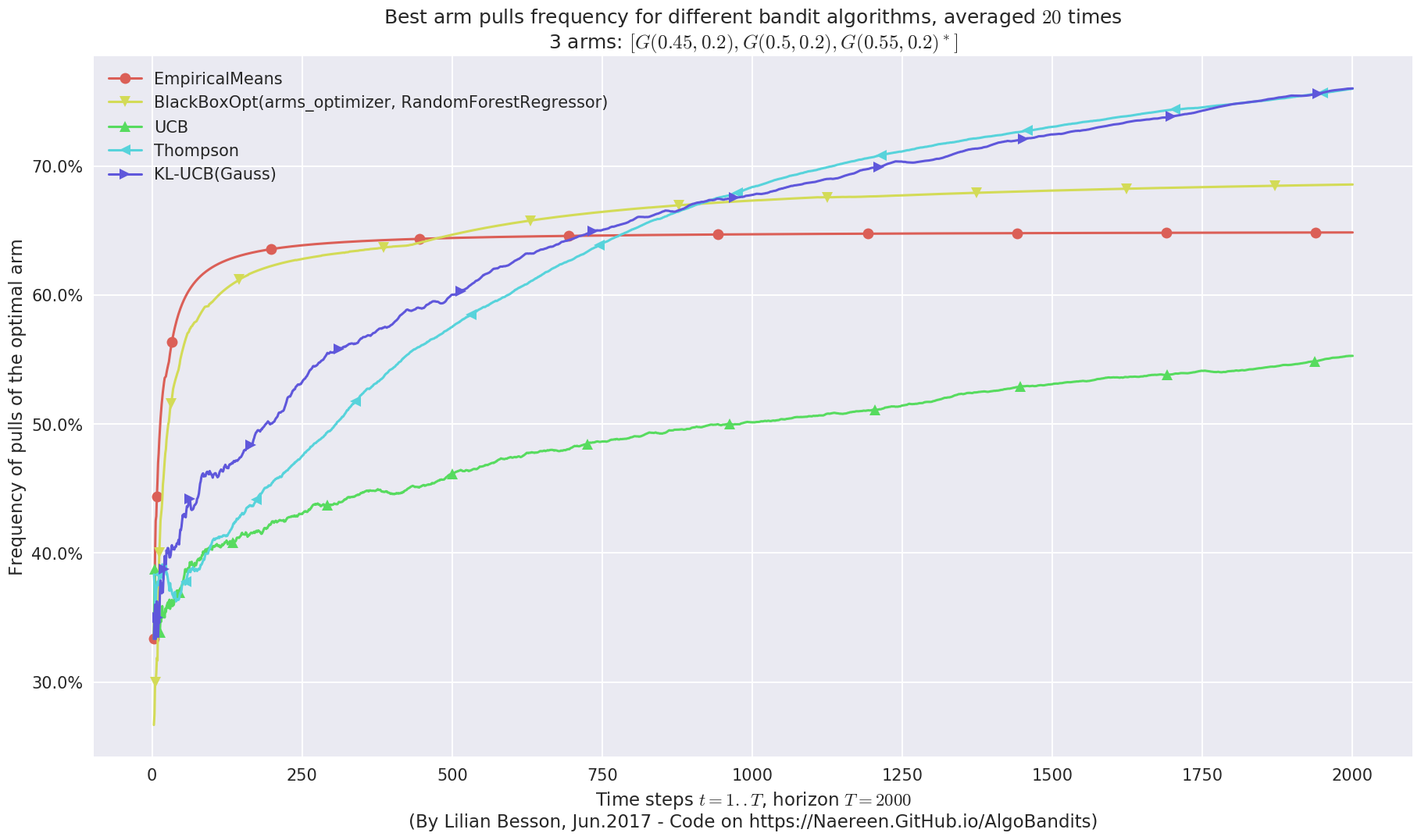
Let create a simple bandit problem, with 3 arms, and visualize an histogram showing the repartition of rewards.

[8]:

means = [0.45, 0.5, 0.55]
M = MAB(Gaussian(mu, sigma=0.2) for mu in means)



Creating a new MAB problem ...
  Taking arms of this MAB problem from a list of arms 'configuration' = <generator object <genexpr> at 0x7f744fca4fc0> ...
 - with 'arms' = [N(0.45, 0.2), N(0.5, 0.2), N(0.55, 0.2)]
 - with 'means' = [0.45 0.5  0.55]
 - with 'nbArms' = 3
 - with 'maxArm' = 0.55
 - with 'minArm' = 0.45

This MAB problem has:
 - a [Lai & Robbins] complexity constant C(mu) = 12 ...
 - a Optimal Arm Identification factor H_OI(mu) = 61.67% ...
 - with 'arms' represented as: $[N(0.45), N(0.5), N(0.55)^*], \sigma^2=0.2$

[9]:

_ = M.plotHistogram(horizon=10000000)

/home/lilian/ownCloud/owncloud.crans.org/Crans/These_2016-17/src/SMPyBandits/notebooks/venv3/lib/python3.6/site-packages/matplotlib/axes/_axes.py:6521: MatplotlibDeprecationWarning:
The 'normed' kwarg was deprecated in Matplotlib 2.1 and will be removed in 3.1. Use 'density' instead.
  alternative="'density'", removal="3.1")

Warning: forcing to use putatright = False because there is 3 items in the legend.

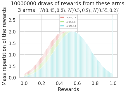
As we can see, the rewards of the different arms are close. It won’t be easy to distinguish them.

Using a Black-Box optimization algorithm¶

I will present directly how to use any black-box optimization algorithm, following `skopt “ask-and-tell” <https://scikit-optimize.github.io/notebooks/ask-and-tell.html>`__ API.

The optimization algorithm, opt, needs two methods:

opt.tell, used like opt.tell([armId], loss), to give an observation of a certain “loss” (loss = - reward) from arm #armId to the algorithm.
opt.ask, used like asked = opt.ask(), to ask the algorithm which arm should be sampled first.

Let use a simple Black-Box Bayesian algorithm, implemented in the scikit-optimize (``skopt`) <https://scikit-optimize.github.io/>`__ package: `RandomForestRegressor <https://scikit-optimize.github.io/learning/index.html#skopt.learning.RandomForestRegressor>`__.

[9]:

from skopt.learning import RandomForestRegressor

First, we need to create a model.

[10]:

our_est = RandomForestRegressor()

[11]:

our_est?

Type:        RandomForestRegressor
String form:
RandomForestRegressor(bootstrap=True, criterion='mse', max_depth=None,
           max_features='a <...> imators=10, n_jobs=1,
           oob_score=False, random_state=None, verbose=0, warm_start=False)
Length:      0
File:        /usr/local/lib/python3.5/dist-packages/skopt/learning/forest.py
Docstring:   RandomForestRegressor that supports `return_std`.

Then the optimization process is using the `Optimizer <https://scikit-optimize.github.io/#skopt.Optimizer>`__ class from `skopt <https://scikit-optimize.github.io/>`__.

[12]:

from skopt import Optimizer

[13]:

def arms_optimizer(nbArms, est):
    return Optimizer([
            list(range(nbArms))  # Categorical dimensions: arm index!
        ],
        est(),
        acq_optimizer="sampling",
        n_random_starts=3 * nbArms  # Sure ?
    )

[14]:

our_opt = arms_optimizer(M.nbArms, RandomForestRegressor)

[15]:

our_opt?

Type:        Optimizer
String form: <skopt.optimizer.optimizer.Optimizer object at 0x7efda4b6a550>
File:        /usr/local/lib/python3.5/dist-packages/skopt/optimizer/optimizer.py
Docstring:
Run bayesian optimisation loop.

An `Optimizer` represents the steps of a bayesian optimisation loop. To
use it you need to provide your own loop mechanism. The various
optimisers provided by `skopt` use this class under the hood.

Use this class directly if you want to control the iterations of your
bayesian optimisation loop.

Parameters
----------
* `dimensions` [list, shape=(n_dims,)]:
    List of search space dimensions.
    Each search dimension can be defined either as

    - a `(upper_bound, lower_bound)` tuple (for `Real` or `Integer`
      dimensions),
    - a `(upper_bound, lower_bound, "prior")` tuple (for `Real`
      dimensions),
    - as a list of categories (for `Categorical` dimensions), or
    - an instance of a `Dimension` object (`Real`, `Integer` or
      `Categorical`).

* `base_estimator` [sklearn regressor]:
    Should inherit from `sklearn.base.RegressorMixin`.
    In addition the `predict` method, should have an optional `return_std`
    argument, which returns `std(Y | x)`` along with `E[Y | x]`.

* `n_random_starts` [int, default=10]:
    Number of evaluations of `func` with random initialization points
    before approximating the `func` with `base_estimator`. While random
    points are being suggested no model will be fit to the observations.

* `acq_func` [string, default=`"EI"`]:
    Function to minimize over the posterior distribution. Can be either

    - `"LCB"` for lower confidence bound.
    - `"EI"` for negative expected improvement.
    - `"PI"` for negative probability of improvement.
    - `"gp_hedge"` Probabilistically choose one of the above three
      acquisition functions at every iteration.
        - The gains `g_i` are initialized to zero.
        - At every iteration,
            - Each acquisition function is optimised independently to propose an
              candidate point `X_i`.
            - Out of all these candidate points, the next point `X_best` is
              chosen by $softmax(\eta g_i)$
            - After fitting the surrogate model with `(X_best, y_best)`,
              the gains are updated such that $g_i -= \mu(X_i)$

* `acq_optimizer` [string, `"sampling"` or `"lbfgs"`, default=`"lbfgs"`]:
    Method to minimize the acquistion function. The fit model
    is updated with the optimal value obtained by optimizing `acq_func`
    with `acq_optimizer`.

    - If set to `"sampling"`, then `acq_func` is optimized by computing
      `acq_func` at `n_points` sampled randomly.
    - If set to `"lbfgs"`, then `acq_func` is optimized by
          - Sampling `n_restarts_optimizer` points randomly.
          - `"lbfgs"` is run for 20 iterations with these points as initial
            points to find local minima.
          - The optimal of these local minima is used to update the prior.

* `random_state` [int, RandomState instance, or None (default)]:
    Set random state to something other than None for reproducible
    results.

* `acq_func_kwargs` [dict]:
    Additional arguments to be passed to the acquistion function.

* `acq_optimizer_kwargs` [dict]:
    Additional arguments to be passed to the acquistion optimizer.

Attributes
----------
* `Xi` [list]:
    Points at which objective has been evaluated.
* `yi` [scalar]:
    Values of objective at corresponding points in `Xi`.
* `models` [list]:
    Regression models used to fit observations and compute acquisition
    function.
* `space`
    An instance of `skopt.space.Space`. Stores parameter search space used
    to sample points, bounds, and type of parameters.

Implementation¶

In code, this gives the following:

the getReward(arm, reward) method gives loss = 1 - reward to the optimization process, with opt.tell method,
the choice() simply calls opt.ask().

Note that the Bayesian optimization takes place with an input space of categorial data: instead of optimizing in \(\mathbb{R}\) or \(\mathbb{R}^K\) (for \(K\) arms), the input space is a categorical representation of \(\{1,\dots,K\}\).

[16]:

class BlackBoxOpt(object):
    """Black-box Bayesian optimizer for Multi-Armed Bandit, using Gaussian processes.

    - **Warning**: still highly experimental! Very slow!
    """

    def __init__(self, nbArms,
                 opt=arms_optimizer, est=RandomForestRegressor,
                 lower=0., amplitude=1.,  # not used, but needed for my framework
                 ):
        self.nbArms = nbArms  #: Number of arms of the MAB problem.
        self.t = -1  #: Current time.
        # Black-box optimizer
        self._opt = opt  # Store it
        self._est = est  # Store it
        self.opt = opt(nbArms, est)  #: The black-box optimizer to use, initialized from the other arguments
        # Other attributes
        self.lower = lower  #: Known lower bounds on the rewards.
        self.amplitude = amplitude  #: Known amplitude of the rewards.

    # --- Easy methods

    def __str__(self):
        return "BlackBoxOpt({}, {})".format(self._opt.__name__, self._est.__name__)

    def startGame(self):
        """ Reinitialize the black-box optimizer."""
        self.t = -1
        self.opt = self._opt(self.nbArms, self._est)  # The black-box optimizer to use, initialized from the other arguments

    def getReward(self, armId, reward):
        """ Store this observation `reward` for that arm `armId`.

        - In fact, :class:`skopt.Optimizer` is a *minimizer*, so `loss=1-reward` is stored, to maximize the rewards by minimizing the losses.
        """
        reward = (reward - self.lower) / self.amplitude  # project the reward to [0, 1]
        loss = 1. - reward  # flip
        return self.opt.tell([armId], loss)

    def choice(self):
        r""" Choose an arm, according to the black-box optimizer."""
        self.t += 1
        asked = self.opt.ask()
        # That's a np.array of int, as we use Categorical input dimension!
        arm = int(np.round(asked[0]))
        return arm

[17]:

BlackBoxOpt?

Init signature: BlackBoxOpt(nbArms, opt=<function arms_optimizer at 0x7efda4b61488>, est=<class 'skopt.learning.forest.RandomForestRegressor'>, lower=0.0, amplitude=1.0)
Docstring:
Black-box Bayesian optimizer for Multi-Armed Bandit, using Gaussian processes.

- **Warning**: still highly experimental! Very slow!
Type:           type

For example, for the problem \(M\) defined above, for \(K=3\) arms, this gives the following policy:

[18]:

policy = BlackBoxOpt(M.nbArms)
policy?

Type:        BlackBoxOpt
String form: BlackBoxOpt(arms_optimizer, RandomForestRegressor)
Docstring:
Black-box Bayesian optimizer for Multi-Armed Bandit, using Gaussian processes.

- **Warning**: still highly experimental! Very slow!

Comparing its performance on this Gaussian problem¶

We can compare the performance of this BlackBoxOpt policy, using Random Forest regression, on the same Gaussian problem, against three strategies:

`EmpiricalMeans <https://smpybandits.github.io/docs/Policies.EmpiricalMeans.html#Policies.EmpiricalMeans.EmpiricalMeans>`__, which only uses the empirical mean estimators \(\hat{\mu_k}(t)\). It is known to be insufficient.
`UCB <https://smpybandits.github.io/docs/Policies.UCB.html#Policies.UCB.UCB>`__, the UCB1 algorithm. It is known to be quite efficient.
`Thompson <https://smpybandits.github.io/docs/Policies.Thompson.html#Policies.Thompson.Thompson>`__, the Thompson Sampling algorithm. It is known to be very efficient.
`klUCB <https://smpybandits.github.io/docs/Policies.klUCB.html#Policies.klUCB.klUCB>`__, the kl-UCB algorithm, for Gaussian arms (klucb = klucbGauss). It is also known to be very efficient.

Configuring an experiment¶

I implemented in the `Environment <http://https://smpybandits.github.io/docs/Environment.html>`__ module an `Evaluator <http://https://smpybandits.github.io/docs/Environment.Evaluator.html#Environment.Evaluator.Evaluator>`__ class, very convenient to run experiments of Multi-Armed Bandit games without a sweat.

Let us use it!

[19]:

from SMPyBandits.Environment import Evaluator

We will start with a small experiment, with a small horizon \(T = 2000\) and only \(20\) repetitions. (we should do more, but it is very slow due to BlackBoxOpt…)

[20]:

HORIZON = 2000
REPETITIONS = 20
N_JOBS = min(REPETITIONS, 3)
means = [0.45, 0.5, 0.55]
ENVIRONMENTS = [ [Gaussian(mu, sigma=0.2) for mu in means] ]

[21]:

from SMPyBandits.Policies import EmpiricalMeans, UCB, Thompson, klUCB
from SMPyBandits.Policies import klucb_mapping, klucbGauss as _klucbGauss

sigma = 0.2
# Custom klucb function
def klucbGauss(x, d, precision=0.):
    """klucbGauss(x, d, sig2) with the good variance (= sigma)."""
    return _klucbGauss(x, d, sigma)

klucb = klucbGauss

Info: numba.jit seems to be available.

[22]:

POLICIES = [
        # --- Naive algorithms
        {
            "archtype": EmpiricalMeans,
            "params": {}
        },
        # --- Our algorithm, with two Unsupervised Learning algorithms
        {
            "archtype": BlackBoxOpt,
            "params": {}
        },
        # --- Basic UCB1 algorithm
        {
            "archtype": UCB,
            "params": {}
        },
        # --- Thompson sampling algorithm
        {
            "archtype": Thompson,
            "params": {}
        },
        # --- klUCB algorithm, with Gaussian klucb function
        {
            "archtype": klUCB,
            "params": {
                "klucb": klucb
            }
        },
    ]

[23]:

configuration = {
    # --- Duration of the experiment
    "horizon": HORIZON,
    # --- Number of repetition of the experiment (to have an average)
    "repetitions": REPETITIONS,
    # --- Parameters for the use of joblib.Parallel
    "n_jobs": N_JOBS,    # = nb of CPU cores
    "verbosity": 6,      # Max joblib verbosity
    # --- Arms
    "environment": ENVIRONMENTS,
    # --- Algorithms
    "policies": POLICIES,
}

[24]:

evaluation = Evaluator(configuration)

Number of policies in this comparison: 5
Time horizon: 2000
Number of repetitions: 20
Sampling rate for saving, delta_t_save: 1
Sampling rate for plotting, delta_t_plot: 1
Number of jobs for parallelization: 3
Creating a new MAB problem ...
  Taking arms of this MAB problem from a list of arms 'configuration' = [G(0.45, 0.2), G(0.5, 0.2), G(0.55, 0.2)] ...
 - with 'arms' = [G(0.45, 0.2), G(0.5, 0.2), G(0.55, 0.2)]
 - with 'means' = [ 0.45  0.5   0.55]
 - with 'nbArms' = 3
 - with 'maxArm' = 0.55
 - with 'minArm' = 0.45

This MAB problem has:
 - a [Lai & Robbins] complexity constant C(mu) = 12 ...
 - a Optimal Arm Identification factor H_OI(mu) = 61.67% ...
 - with 'arms' represented as: $[G(0.45, 0.2), G(0.5, 0.2), G(0.55, 0.2)^*]$
Number of environments to try: 1

Running an experiment¶

We asked to repeat the experiment \(20\) times, so it will take a while… (about 100 minutes maximum).

[25]:

from SMPyBandits.Environment import tqdm  # just a pretty loop

[26]:

%%time
for envId, env in tqdm(enumerate(evaluation.envs), desc="Problems"):
    # Evaluate just that env
    evaluation.startOneEnv(envId, env)


Evaluating environment: MAB(nbArms: 3, arms: [G(0.45, 0.2), G(0.5, 0.2), G(0.55, 0.2)], minArm: 0.45, maxArm: 0.55)
- Adding policy #1 = {'archtype': <class 'Policies.EmpiricalMeans.EmpiricalMeans'>, 'params': {}} ...
  Creating this policy from a dictionnary 'self.cfg['policies'][0]' = {'archtype': <class 'Policies.EmpiricalMeans.EmpiricalMeans'>, 'params': {}} ...
- Adding policy #2 = {'archtype': <class '__main__.BlackBoxOpt'>, 'params': {}} ...
  Creating this policy from a dictionnary 'self.cfg['policies'][1]' = {'archtype': <class '__main__.BlackBoxOpt'>, 'params': {}} ...
- Adding policy #3 = {'archtype': <class 'Policies.UCB.UCB'>, 'params': {}} ...
  Creating this policy from a dictionnary 'self.cfg['policies'][2]' = {'archtype': <class 'Policies.UCB.UCB'>, 'params': {}} ...
- Adding policy #4 = {'archtype': <class 'Policies.Thompson.Thompson'>, 'params': {}} ...
  Creating this policy from a dictionnary 'self.cfg['policies'][3]' = {'archtype': <class 'Policies.Thompson.Thompson'>, 'params': {}} ...
- Adding policy #5 = {'archtype': <class 'Policies.klUCB.klUCB'>, 'params': {'klucb': <function klucbGauss at 0x7efdb30d0268>}} ...
  Creating this policy from a dictionnary 'self.cfg['policies'][4]' = {'archtype': <class 'Policies.klUCB.klUCB'>, 'params': {'klucb': <function klucbGauss at 0x7efdb30d0268>}} ...

- Evaluating policy #1/5: EmpiricalMeans ...


Estimated order by the policy EmpiricalMeans after 2000 steps: [1 0 2] ...
  ==> Optimal arm identification: 100.00% (relative success)...
  ==> Manhattan   distance from optimal ordering: 55.56% (relative success)...
  ==> Kendell Tau distance from optimal ordering: 39.85% (relative success)...
  ==> Spearman    distance from optimal ordering: 33.33% (relative success)...
  ==> Gestalt     distance from optimal ordering: 66.67% (relative success)...
  ==> Mean distance from optimal ordering: 48.85% (relative success)...

- Evaluating policy #2/5: BlackBoxOpt(arms_optimizer, RandomForestRegressor) ...

[Parallel(n_jobs=3)]: Done  20 out of  20 | elapsed:    0.6s finished

[Parallel(n_jobs=3)]: Done   7 tasks      | elapsed: 14.5min


- Evaluating policy #3/5: UCB ...

[Parallel(n_jobs=3)]: Done  20 out of  20 | elapsed: 33.6min finished


Estimated order by the policy UCB after 2000 steps: [1 0 2] ...
  ==> Optimal arm identification: 100.00% (relative success)...
  ==> Manhattan   distance from optimal ordering: 55.56% (relative success)...
  ==> Kendell Tau distance from optimal ordering: 39.85% (relative success)...
  ==> Spearman    distance from optimal ordering: 33.33% (relative success)...
  ==> Gestalt     distance from optimal ordering: 66.67% (relative success)...
  ==> Mean distance from optimal ordering: 48.85% (relative success)...

- Evaluating policy #4/5: Thompson ...

[Parallel(n_jobs=3)]: Done  20 out of  20 | elapsed:    0.6s finished


Estimated order by the policy Thompson after 2000 steps: [1 2 0] ...
  ==> Optimal arm identification: 81.82% (relative success)...
  ==> Manhattan   distance from optimal ordering: 11.11% (relative success)...
  ==> Kendell Tau distance from optimal ordering: 39.85% (relative success)...
  ==> Spearman    distance from optimal ordering: 33.33% (relative success)...
  ==> Gestalt     distance from optimal ordering: 66.67% (relative success)...
  ==> Mean distance from optimal ordering: 37.74% (relative success)...

- Evaluating policy #5/5: KL-UCB(Gauss) ...

[Parallel(n_jobs=3)]: Done  20 out of  20 | elapsed:    0.6s finished


Estimated order by the policy KL-UCB(Gauss) after 2000 steps: [0 1 2] ...
  ==> Optimal arm identification: 100.00% (relative success)...
  ==> Manhattan   distance from optimal ordering: 100.00% (relative success)...
  ==> Kendell Tau distance from optimal ordering: 88.28% (relative success)...
  ==> Spearman    distance from optimal ordering: 100.00% (relative success)...
  ==> Gestalt     distance from optimal ordering: 100.00% (relative success)...
  ==> Mean distance from optimal ordering: 97.07% (relative success)...

[Parallel(n_jobs=3)]: Done   7 tasks      | elapsed:    0.9s


CPU times: user 1.57 s, sys: 464 ms, total: 2.04 s
Wall time: 33min 42s

[Parallel(n_jobs=3)]: Done  20 out of  20 | elapsed:    2.0s finished

Visualizing the results¶

Now, we can plot some performance measures, like the regret, the best arm selection rate, the average reward etc.

[27]:

def plotAll(evaluation, envId=0):
    evaluation.printFinalRanking(envId)
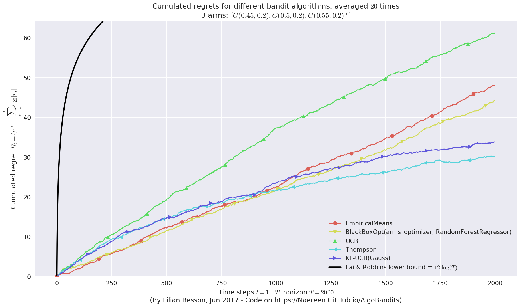
    evaluation.plotRegrets(envId)
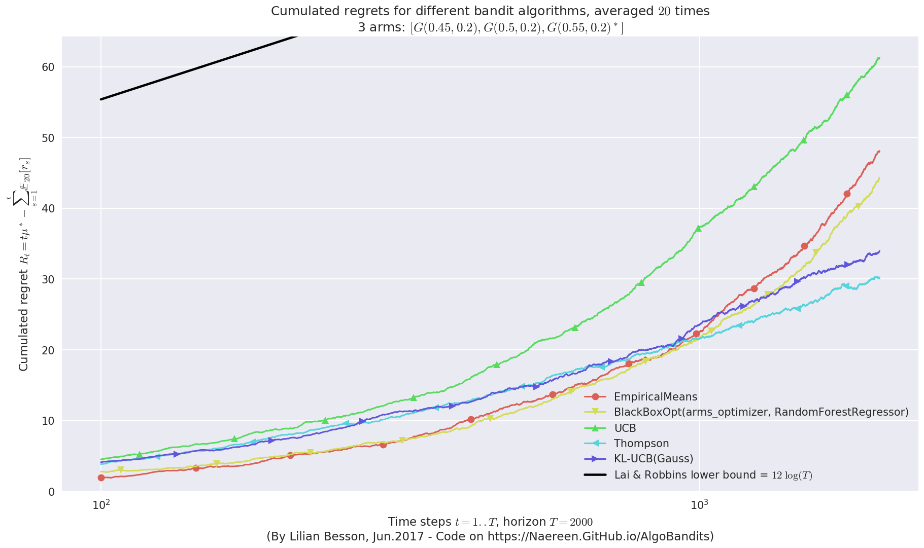
    evaluation.plotRegrets(envId, semilogx=True)
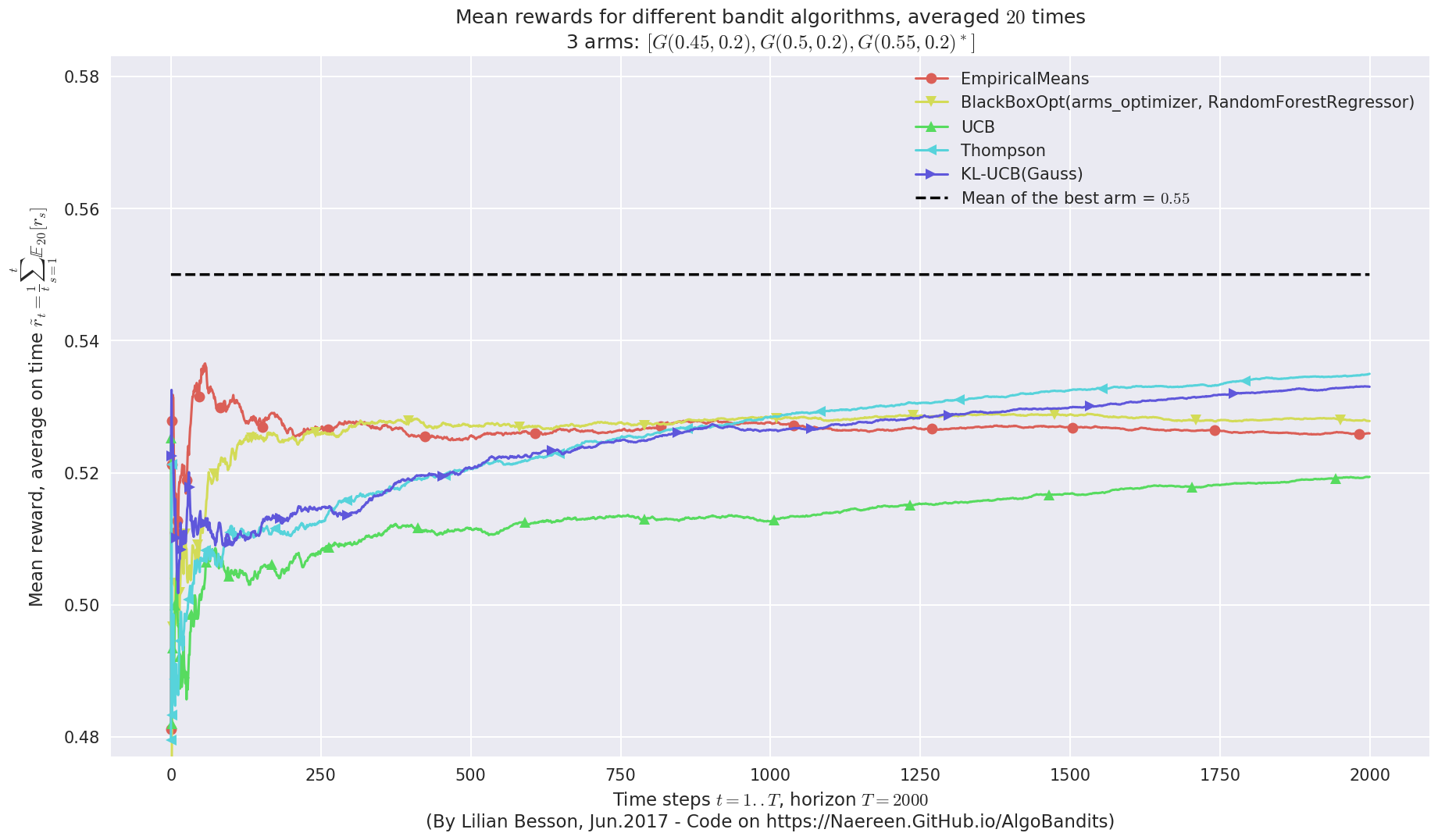
    evaluation.plotRegrets(envId, meanRegret=True)
    evaluation.plotBestArmPulls(envId)

[28]:

evaluation?

Type:        Evaluator
String form: <Environment.Evaluator.Evaluator object at 0x7efda4b6aac8>
File:        ~/ownCloud/cloud.openmailbox.org/Thèse_2016-17/src/SMPyBandits.git/Environment/Evaluator.py
Docstring:   Evaluator class to run the simulations.

[29]:

plotAll(evaluation)


Final ranking for this environment #0 :
- Policy 'Thompson'     was ranked      1 / 5 for this simulation (last regret = 30.2294).
- Policy 'KL-UCB(Gauss)'        was ranked      2 / 5 for this simulation (last regret = 33.7103).
- Policy 'BlackBoxOpt(arms_optimizer, RandomForestRegressor)'   was ranked      3 / 5 for this simulation (last regret = 43.7773).
- Policy 'EmpiricalMeans'       was ranked      4 / 5 for this simulation (last regret = 48.0636).
- Policy 'UCB'  was ranked      5 / 5 for this simulation (last regret = 61.1631).

This MAB problem has:
 - a [Lai & Robbins] complexity constant C(mu) = 12 for 1-player problem...
 - a Optimal Arm Identification factor H_OI(mu) = 61.67% ...

../_images/notebooks_BlackBox_Bayesian_Optimization_for_Bandit_problems_44_1.png


This MAB problem has:
 - a [Lai & Robbins] complexity constant C(mu) = 12 for 1-player problem...
 - a Optimal Arm Identification factor H_OI(mu) = 61.67% ...

../_images/notebooks_BlackBox_Bayesian_Optimization_for_Bandit_problems_44_3.png


This MAB problem has:
 - a [Lai & Robbins] complexity constant C(mu) = 12 for 1-player problem...
 - a Optimal Arm Identification factor H_OI(mu) = 61.67% ...

../_images/notebooks_BlackBox_Bayesian_Optimization_for_Bandit_problems_44_5.png

../_images/notebooks_BlackBox_Bayesian_Optimization_for_Bandit_problems_44_6.png

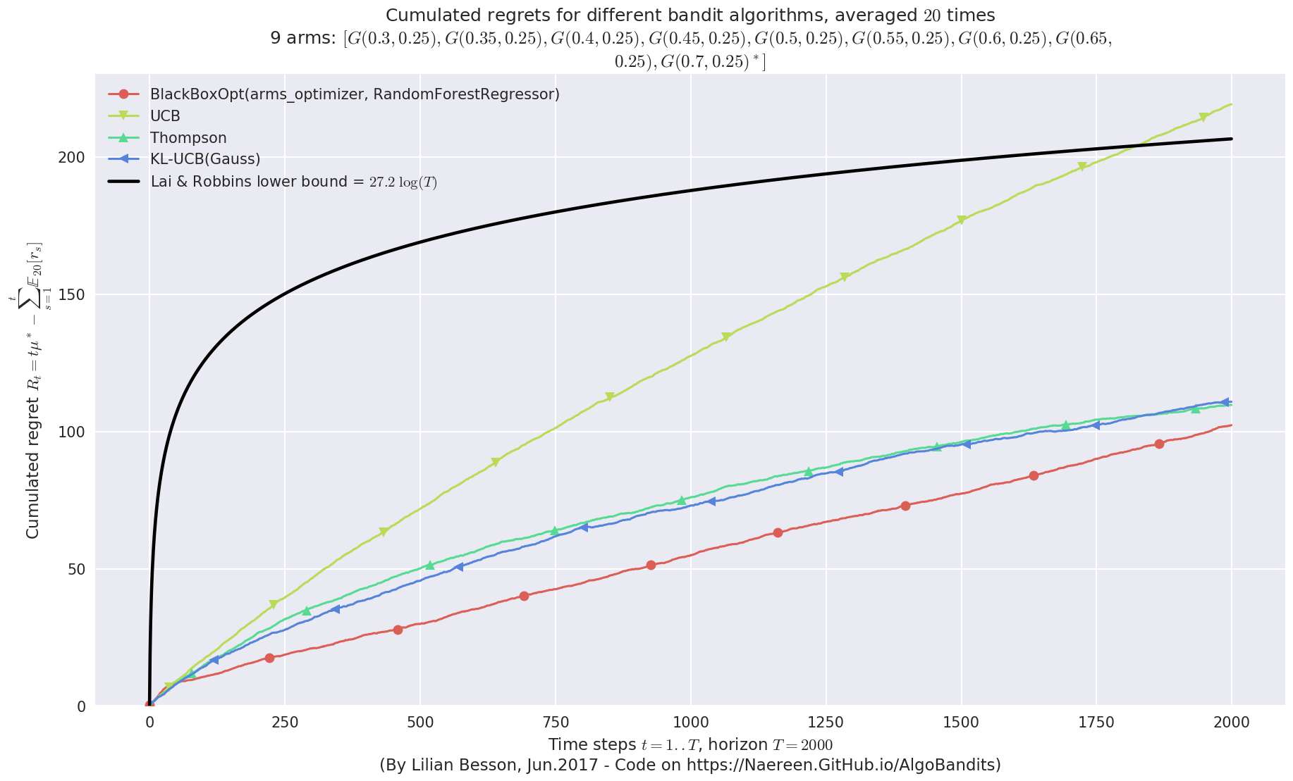
Another experiment, with just more Gaussian arms¶

This second experiment will be similar, except we consider more arms. As they are all very close to each other, with a gap \(\Delta = 0.05\), it gets much harder!

[30]:

HORIZON = 2000
REPETITIONS = 20
N_JOBS = min(REPETITIONS, 4)
means = [0.30, 0.35, 0.40, 0.45, 0.5, 0.55, 0.60, 0.65, 0.70]
ENVIRONMENTS = [ [Gaussian(mu, sigma=0.25) for mu in means] ]

[31]:

POLICIES = [
        # --- Our algorithm, with two Unsupervised Learning algorithms
        {
            "archtype": BlackBoxOpt,
            "params": {}
        },
        # --- Basic UCB1 algorithm
        {
            "archtype": UCB,
            "params": {}
        },
        # --- Thompson sampling algorithm
        {
            "archtype": Thompson,
            "params": {}
        },
        # --- klUCB algorithm, with Gaussian klucb function
        {
            "archtype": klUCB,
            "params": {
                "klucb": klucb
            }
        },
    ]

[32]:

configuration = {
    # --- Duration of the experiment
    "horizon": HORIZON,
    # --- Number of repetition of the experiment (to have an average)
    "repetitions": REPETITIONS,
    # --- Parameters for the use of joblib.Parallel
    "n_jobs": N_JOBS,    # = nb of CPU cores
    "verbosity": 6,      # Max joblib verbosity
    # --- Arms
    "environment": ENVIRONMENTS,
    # --- Algorithms
    "policies": POLICIES,
}

[33]:

evaluation2 = Evaluator(configuration)

Number of policies in this comparison: 4
Time horizon: 2000
Number of repetitions: 20
Sampling rate for saving, delta_t_save: 1
Sampling rate for plotting, delta_t_plot: 1
Number of jobs for parallelization: 4
Creating a new MAB problem ...
  Taking arms of this MAB problem from a list of arms 'configuration' = [G(0.3, 0.25), G(0.35, 0.25), G(0.4, 0.25), G(0.45, 0.25), G(0.5, 0.25), G(0.55, 0.25), G(0.6, 0.25), G(0.65, 0.25), G(0.7, 0.25)] ...
 - with 'arms' = [G(0.3, 0.25), G(0.35, 0.25), G(0.4, 0.25), G(0.45, 0.25), G(0.5, 0.25), G(0.55, 0.25), G(0.6, 0.25), G(0.65, 0.25), G(0.7, 0.25)]
 - with 'means' = [ 0.3   0.35  0.4   0.45  0.5   0.55  0.6   0.65  0.7 ]
 - with 'nbArms' = 9
 - with 'maxArm' = 0.7
 - with 'minArm' = 0.3

This MAB problem has:
 - a [Lai & Robbins] complexity constant C(mu) = 27.2 ...
 - a Optimal Arm Identification factor H_OI(mu) = 68.89% ...
 - with 'arms' represented as: $[G(0.3, 0.25), G(0.35, 0.25), G(0.4, 0.25), G(0.45, 0.25), G(0.5, 0.25), G(0.55, 0.25), G(0.6, 0.25), G(0.65,$
$0.25), G(0.7, 0.25)^*]$
Number of environments to try: 1

Running the experiment¶

We asked to repeat the experiment \(20\) times, so it will take a while…

[34]:

%%time
for envId, env in tqdm(enumerate(evaluation2.envs), desc="Problems"):
    # Evaluate just that env
    evaluation2.startOneEnv(envId, env)


Evaluating environment: MAB(nbArms: 9, arms: [G(0.3, 0.25), G(0.35, 0.25), G(0.4, 0.25), G(0.45, 0.25), G(0.5, 0.25), G(0.55, 0.25), G(0.6, 0.25), G(0.65, 0.25), G(0.7, 0.25)], minArm: 0.3, maxArm: 0.7)
- Adding policy #1 = {'archtype': <class '__main__.BlackBoxOpt'>, 'params': {}} ...
  Creating this policy from a dictionnary 'self.cfg['policies'][0]' = {'archtype': <class '__main__.BlackBoxOpt'>, 'params': {}} ...
- Adding policy #2 = {'archtype': <class 'Policies.UCB.UCB'>, 'params': {}} ...
  Creating this policy from a dictionnary 'self.cfg['policies'][1]' = {'archtype': <class 'Policies.UCB.UCB'>, 'params': {}} ...
- Adding policy #3 = {'archtype': <class 'Policies.Thompson.Thompson'>, 'params': {}} ...
  Creating this policy from a dictionnary 'self.cfg['policies'][2]' = {'archtype': <class 'Policies.Thompson.Thompson'>, 'params': {}} ...
- Adding policy #4 = {'archtype': <class 'Policies.klUCB.klUCB'>, 'params': {'klucb': <function klucbGauss at 0x7efdb30d0268>}} ...
  Creating this policy from a dictionnary 'self.cfg['policies'][3]' = {'archtype': <class 'Policies.klUCB.klUCB'>, 'params': {'klucb': <function klucbGauss at 0x7efdb30d0268>}} ...

- Evaluating policy #1/4: BlackBoxOpt(arms_optimizer, RandomForestRegressor) ...

[Parallel(n_jobs=4)]: Done   5 tasks      | elapsed: 15.4min
[Parallel(n_jobs=4)]: Done  17 out of  20 | elapsed: 36.7min remaining:  6.5min


- Evaluating policy #2/4: UCB ...

[Parallel(n_jobs=4)]: Done  20 out of  20 | elapsed: 36.9min finished


Estimated order by the policy UCB after 2000 steps: [3 0 1 8 2 5 4 7 6] ...
  ==> Optimal arm identification: 85.71% (relative success)...
  ==> Manhattan   distance from optimal ordering: 60.49% (relative success)...
  ==> Kendell Tau distance from optimal ordering: 90.47% (relative success)...
  ==> Spearman    distance from optimal ordering: 91.24% (relative success)...
  ==> Gestalt     distance from optimal ordering: 33.33% (relative success)...
  ==> Mean distance from optimal ordering: 68.88% (relative success)...

[Parallel(n_jobs=4)]: Done   5 tasks      | elapsed:    0.2s


- Evaluating policy #3/4: Thompson ...

[Parallel(n_jobs=4)]: Done  20 out of  20 | elapsed:    0.6s finished


Estimated order by the policy Thompson after 2000 steps: [5 1 2 4 0 3 6 7 8] ...
  ==> Optimal arm identification: 100.00% (relative success)...
  ==> Manhattan   distance from optimal ordering: 70.37% (relative success)...
  ==> Kendell Tau distance from optimal ordering: 93.94% (relative success)...
  ==> Spearman    distance from optimal ordering: 92.31% (relative success)...
  ==> Gestalt     distance from optimal ordering: 66.67% (relative success)...
  ==> Mean distance from optimal ordering: 80.82% (relative success)...

[Parallel(n_jobs=4)]: Done   5 tasks      | elapsed:    0.3s


- Evaluating policy #4/4: KL-UCB(Gauss) ...

[Parallel(n_jobs=4)]: Done  20 out of  20 | elapsed:    0.7s finished


Estimated order by the policy KL-UCB(Gauss) after 2000 steps: [3 4 1 2 0 6 7 5 8] ...
  ==> Optimal arm identification: 100.00% (relative success)...
  ==> Manhattan   distance from optimal ordering: 60.49% (relative success)...
  ==> Kendell Tau distance from optimal ordering: 90.47% (relative success)...
  ==> Spearman    distance from optimal ordering: 94.19% (relative success)...
  ==> Gestalt     distance from optimal ordering: 55.56% (relative success)...
  ==> Mean distance from optimal ordering: 75.18% (relative success)...

[Parallel(n_jobs=4)]: Done   5 tasks      | elapsed:    0.5s


CPU times: user 1.58 s, sys: 508 ms, total: 2.09 s
Wall time: 36min 56s

[Parallel(n_jobs=4)]: Done  17 out of  20 | elapsed:    1.2s remaining:    0.2s
[Parallel(n_jobs=4)]: Done  20 out of  20 | elapsed:    1.3s finished

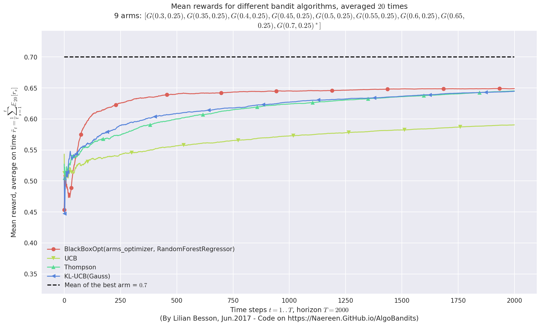
Visualizing the results¶

Now, we can plot some performance measures, like the regret, the best arm selection rate, the average reward etc.

[35]:

plotAll(evaluation2)


Final ranking for this environment #0 :
- Policy 'BlackBoxOpt(arms_optimizer, RandomForestRegressor)'   was ranked      1 / 4 for this simulation (last regret = 101.943).
- Policy 'Thompson'     was ranked      2 / 4 for this simulation (last regret = 109.463).
- Policy 'KL-UCB(Gauss)'        was ranked      3 / 4 for this simulation (last regret = 110.81).
- Policy 'UCB'  was ranked      4 / 4 for this simulation (last regret = 218.572).

This MAB problem has:
 - a [Lai & Robbins] complexity constant C(mu) = 27.2 for 1-player problem...
 - a Optimal Arm Identification factor H_OI(mu) = 68.89% ...

../_images/notebooks_BlackBox_Bayesian_Optimization_for_Bandit_problems_54_1.png


This MAB problem has:
 - a [Lai & Robbins] complexity constant C(mu) = 27.2 for 1-player problem...
 - a Optimal Arm Identification factor H_OI(mu) = 68.89% ...

../_images/notebooks_BlackBox_Bayesian_Optimization_for_Bandit_problems_54_3.png


This MAB problem has:
 - a [Lai & Robbins] complexity constant C(mu) = 27.2 for 1-player problem...
 - a Optimal Arm Identification factor H_OI(mu) = 68.89% ...

../_images/notebooks_BlackBox_Bayesian_Optimization_for_Bandit_problems_54_5.png

../_images/notebooks_BlackBox_Bayesian_Optimization_for_Bandit_problems_54_6.png

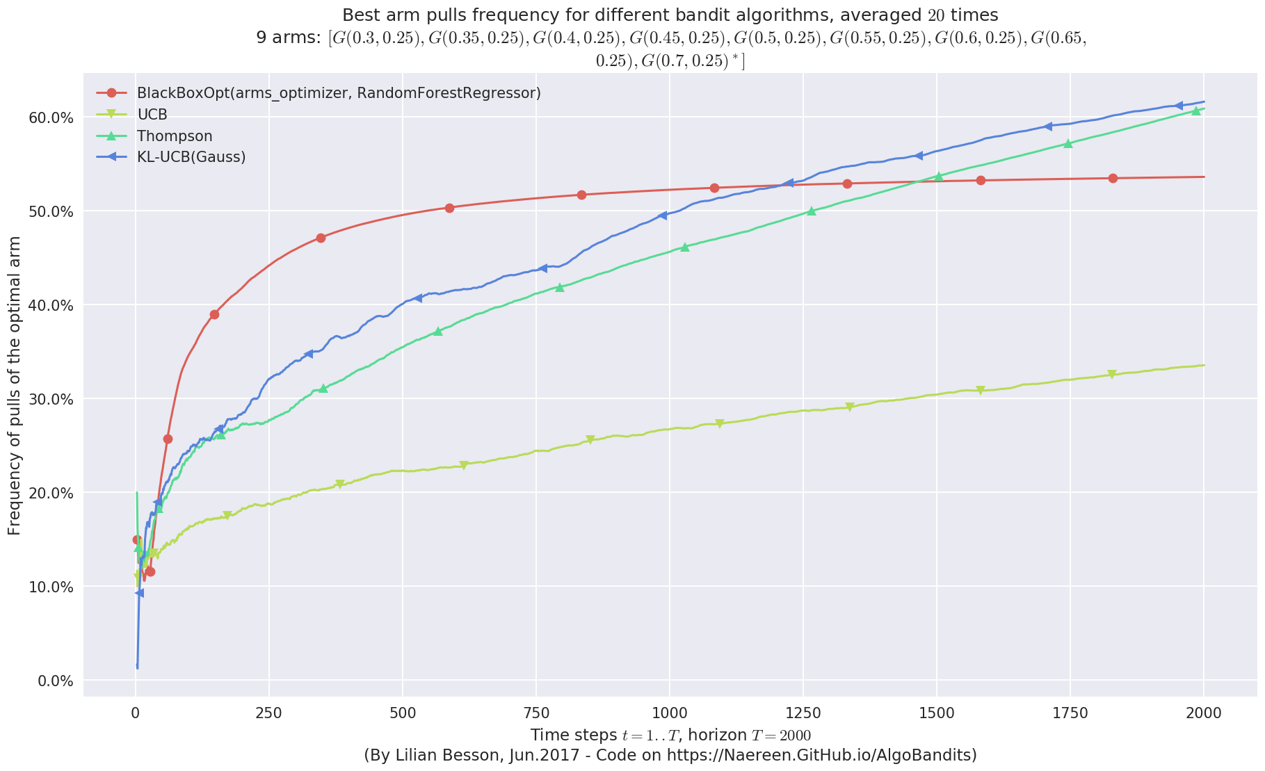
Very good performance!¶

Whoo, on this last experiment, the BlackBoxOpt policy works way better than the three other policies !!

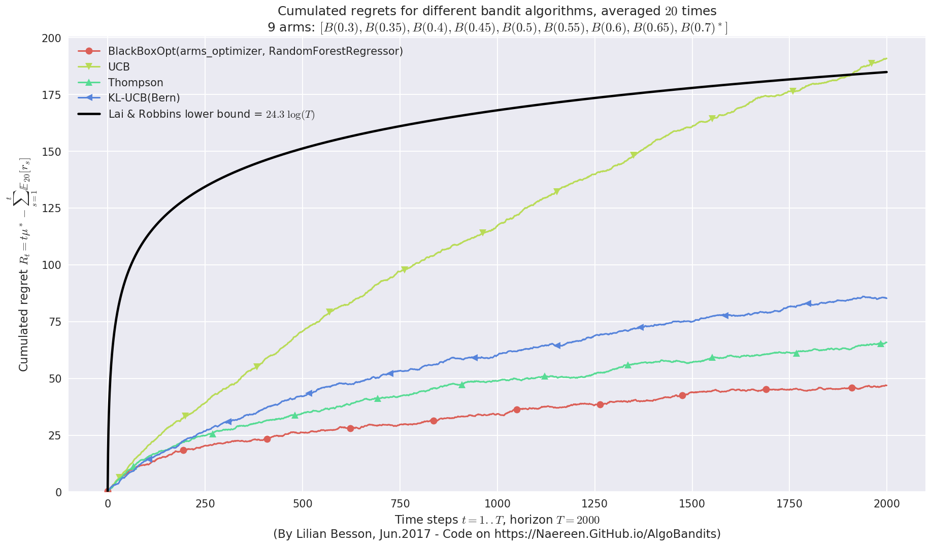
Another experiment, with Bernoulli arms¶

Let also try the same algorithms but on Bernoulli arms.

[36]:

from SMPyBandits.Arms import Bernoulli

[37]:

HORIZON = 2000
REPETITIONS = 20
N_JOBS = min(REPETITIONS, 4)
means = [0.30, 0.35, 0.40, 0.45, 0.5, 0.55, 0.60, 0.65, 0.70]
ENVIRONMENTS = [ [Bernoulli(mu) for mu in means] ]

[42]:

klucbBern = klucb_mapping['Bernoulli']

POLICIES = [
        # --- Our algorithm, with two Unsupervised Learning algorithms
        {
            "archtype": BlackBoxOpt,
            "params": {}
        },
        # --- Basic UCB1 algorithm
        {
            "archtype": UCB,
            "params": {}
        },
        # --- Thompson sampling algorithm
        {
            "archtype": Thompson,
            "params": {}
        },
        # --- klUCB algorithm, with Bernoulli klucb function
        # https://smpybandits.github.io/docs/Arms.kullback.html#Arms.kullback.klucbBern
        {
            "archtype": klUCB,
            "params": {
                "klucb": klucbBern
            }
        },
    ]

[43]:

configuration = {
    # --- Duration of the experiment
    "horizon": HORIZON,
    # --- Number of repetition of the experiment (to have an average)
    "repetitions": REPETITIONS,
    # --- Parameters for the use of joblib.Parallel
    "n_jobs": N_JOBS,    # = nb of CPU cores
    "verbosity": 6,      # Max joblib verbosity
    # --- Arms
    "environment": ENVIRONMENTS,
    # --- Algorithms
    "policies": POLICIES,
}

[44]:

evaluation3 = Evaluator(configuration)

Number of policies in this comparison: 4
Time horizon: 2000
Number of repetitions: 20
Sampling rate for saving, delta_t_save: 1
Sampling rate for plotting, delta_t_plot: 1
Number of jobs for parallelization: 4
Creating a new MAB problem ...
  Taking arms of this MAB problem from a list of arms 'configuration' = [B(0.3), B(0.35), B(0.4), B(0.45), B(0.5), B(0.55), B(0.6), B(0.65), B(0.7)] ...
 - with 'arms' = [B(0.3), B(0.35), B(0.4), B(0.45), B(0.5), B(0.55), B(0.6), B(0.65), B(0.7)]
 - with 'means' = [ 0.3   0.35  0.4   0.45  0.5   0.55  0.6   0.65  0.7 ]
 - with 'nbArms' = 9
 - with 'maxArm' = 0.7
 - with 'minArm' = 0.3

This MAB problem has:
 - a [Lai & Robbins] complexity constant C(mu) = 24.3 ...
 - a Optimal Arm Identification factor H_OI(mu) = 68.89% ...
 - with 'arms' represented as: $[B(0.3), B(0.35), B(0.4), B(0.45), B(0.5), B(0.55), B(0.6), B(0.65), B(0.7)^*]$
Number of environments to try: 1

Running the experiment¶

We asked to repeat the experiment \(20\) times, so it will take a while…

[45]:

%%time
for envId, env in tqdm(enumerate(evaluation3.envs), desc="Problems"):
    # Evaluate just that env
    evaluation3.startOneEnv(envId, env)


Evaluating environment: MAB(nbArms: 9, arms: [B(0.3), B(0.35), B(0.4), B(0.45), B(0.5), B(0.55), B(0.6), B(0.65), B(0.7)], minArm: 0.3, maxArm: 0.7)
- Adding policy #1 = {'archtype': <class '__main__.BlackBoxOpt'>, 'params': {}} ...
  Creating this policy from a dictionnary 'self.cfg['policies'][0]' = {'archtype': <class '__main__.BlackBoxOpt'>, 'params': {}} ...
- Adding policy #2 = {'archtype': <class 'Policies.UCB.UCB'>, 'params': {}} ...
  Creating this policy from a dictionnary 'self.cfg['policies'][1]' = {'archtype': <class 'Policies.UCB.UCB'>, 'params': {}} ...
- Adding policy #3 = {'archtype': <class 'Policies.Thompson.Thompson'>, 'params': {}} ...
  Creating this policy from a dictionnary 'self.cfg['policies'][2]' = {'archtype': <class 'Policies.Thompson.Thompson'>, 'params': {}} ...
- Adding policy #4 = {'archtype': <class 'Policies.klUCB.klUCB'>, 'params': {'klucb': <built-in function klucbBern>}} ...
  Creating this policy from a dictionnary 'self.cfg['policies'][3]' = {'archtype': <class 'Policies.klUCB.klUCB'>, 'params': {'klucb': <built-in function klucbBern>}} ...

- Evaluating policy #1/4: BlackBoxOpt(arms_optimizer, RandomForestRegressor) ...

[Parallel(n_jobs=4)]: Done   5 tasks      | elapsed: 15.2min
[Parallel(n_jobs=4)]: Done  17 out of  20 | elapsed: 35.6min remaining:  6.3min


- Evaluating policy #2/4: UCB ...

[Parallel(n_jobs=4)]: Done  20 out of  20 | elapsed: 36.0min finished


Estimated order by the policy UCB after 2000 steps: [0 4 3 2 1 6 5 8 7] ...
  ==> Optimal arm identification: 92.86% (relative success)...
  ==> Manhattan   distance from optimal ordering: 70.37% (relative success)...
  ==> Kendell Tau distance from optimal ordering: 96.29% (relative success)...
  ==> Spearman    distance from optimal ordering: 99.04% (relative success)...
  ==> Gestalt     distance from optimal ordering: 44.44% (relative success)...
  ==> Mean distance from optimal ordering: 77.54% (relative success)...

[Parallel(n_jobs=4)]: Done   5 tasks      | elapsed:    0.3s


- Evaluating policy #3/4: Thompson ...

[Parallel(n_jobs=4)]: Done  20 out of  20 | elapsed:    0.8s finished


Estimated order by the policy Thompson after 2000 steps: [0 3 1 4 6 5 2 7 8] ...
  ==> Optimal arm identification: 100.00% (relative success)...
  ==> Manhattan   distance from optimal ordering: 75.31% (relative success)...
  ==> Kendell Tau distance from optimal ordering: 98.77% (relative success)...
  ==> Spearman    distance from optimal ordering: 98.75% (relative success)...
  ==> Gestalt     distance from optimal ordering: 66.67% (relative success)...
  ==> Mean distance from optimal ordering: 84.87% (relative success)...

[Parallel(n_jobs=4)]: Done   5 tasks      | elapsed:    0.3s


- Evaluating policy #4/4: KL-UCB(Bern) ...

[Parallel(n_jobs=4)]: Done  20 out of  20 | elapsed:    0.9s finished


Estimated order by the policy KL-UCB(Bern) after 2000 steps: [0 2 1 4 3 5 6 7 8] ...
  ==> Optimal arm identification: 100.00% (relative success)...
  ==> Manhattan   distance from optimal ordering: 90.12% (relative success)...
  ==> Kendell Tau distance from optimal ordering: 99.92% (relative success)...
  ==> Spearman    distance from optimal ordering: 100.00% (relative success)...
  ==> Gestalt     distance from optimal ordering: 77.78% (relative success)...
  ==> Mean distance from optimal ordering: 91.95% (relative success)...

[Parallel(n_jobs=4)]: Done   5 tasks      | elapsed:    0.5s


CPU times: user 1.5 s, sys: 560 ms, total: 2.06 s
Wall time: 36min 5s

[Parallel(n_jobs=4)]: Done  17 out of  20 | elapsed:    1.6s remaining:    0.3s
[Parallel(n_jobs=4)]: Done  20 out of  20 | elapsed:    1.7s finished

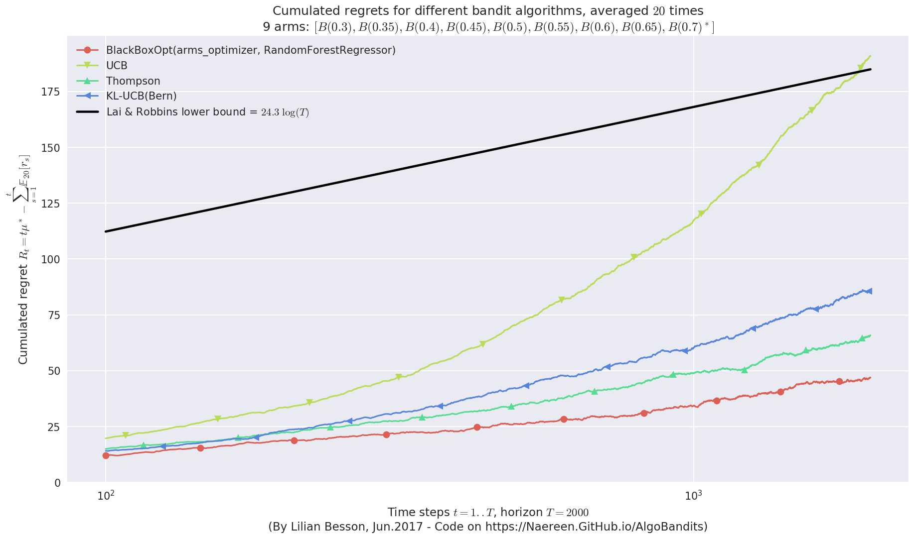
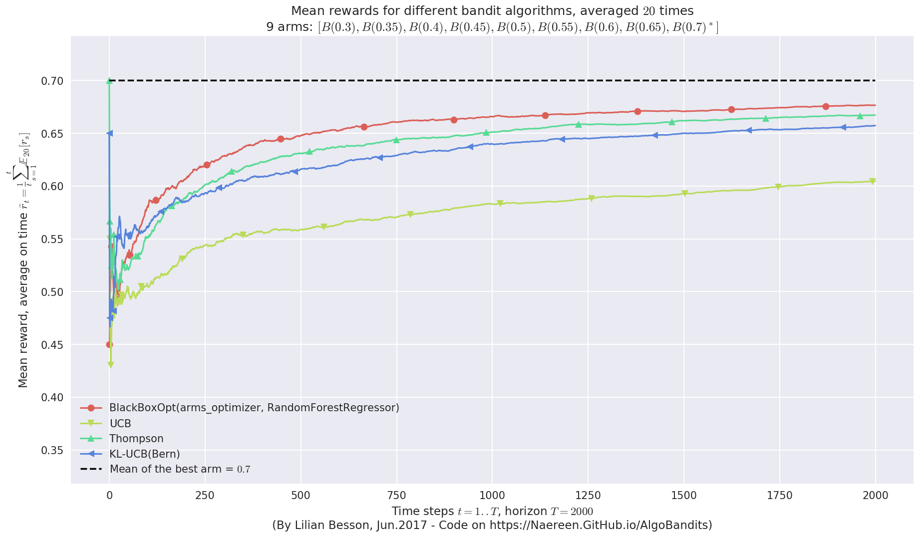
Visualizing the results¶

Now, we can plot some performance measures, like the regret, the best arm selection rate, the average reward etc.

[46]:

plotAll(evaluation3)


Final ranking for this environment #0 :
- Policy 'BlackBoxOpt(arms_optimizer, RandomForestRegressor)'   was ranked      1 / 4 for this simulation (last regret = 46.7).
- Policy 'Thompson'     was ranked      2 / 4 for this simulation (last regret = 65.35).
- Policy 'KL-UCB(Bern)' was ranked      3 / 4 for this simulation (last regret = 85.6).
- Policy 'UCB'  was ranked      4 / 4 for this simulation (last regret = 190.35).

This MAB problem has:
 - a [Lai & Robbins] complexity constant C(mu) = 24.3 for 1-player problem...
 - a Optimal Arm Identification factor H_OI(mu) = 68.89% ...

../_images/notebooks_BlackBox_Bayesian_Optimization_for_Bandit_problems_65_1.png


This MAB problem has:
 - a [Lai & Robbins] complexity constant C(mu) = 24.3 for 1-player problem...
 - a Optimal Arm Identification factor H_OI(mu) = 68.89% ...

../_images/notebooks_BlackBox_Bayesian_Optimization_for_Bandit_problems_65_3.png


This MAB problem has:
 - a [Lai & Robbins] complexity constant C(mu) = 24.3 for 1-player problem...
 - a Optimal Arm Identification factor H_OI(mu) = 68.89% ...

../_images/notebooks_BlackBox_Bayesian_Optimization_for_Bandit_problems_65_5.png

../_images/notebooks_BlackBox_Bayesian_Optimization_for_Bandit_problems_65_6.png

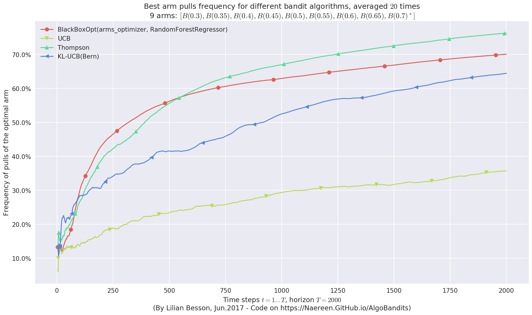
Very good performances also!¶

We can see that BlackBoxOpt with RandomForestRegressor also has very good performances on Bernoulli problems!

Conclusion¶

This small simulation shows that with the appropriate tweaking of parameters, and on reasonably easy Gaussian Multi-Armed Bandit problems, one can use a Black-Box Bayesian optimization algorithm, with an “ask-and-tell” API to make it on-line.

Without the need of any parameter tweaking or model selection steps, the BlackBoxOpt policy was quite efficient (using the default `Optimizer <https://scikit-optimize.github.io/learning/index.html#skopt.Optimizer>`__ and the `RandomForestRegressor <https://scikit-optimize.github.io/index.html#skopt.learning.RandomForestRegressor>`__, from `skopt <https://scikit-optimize.github.io/>`__ package).

When comparing in terms of mean rewards, accumulated rewards, best-arm selection, and regret (loss against the best fixed-arm policy), this BlackBoxOpt algorithm performs as well as the others.

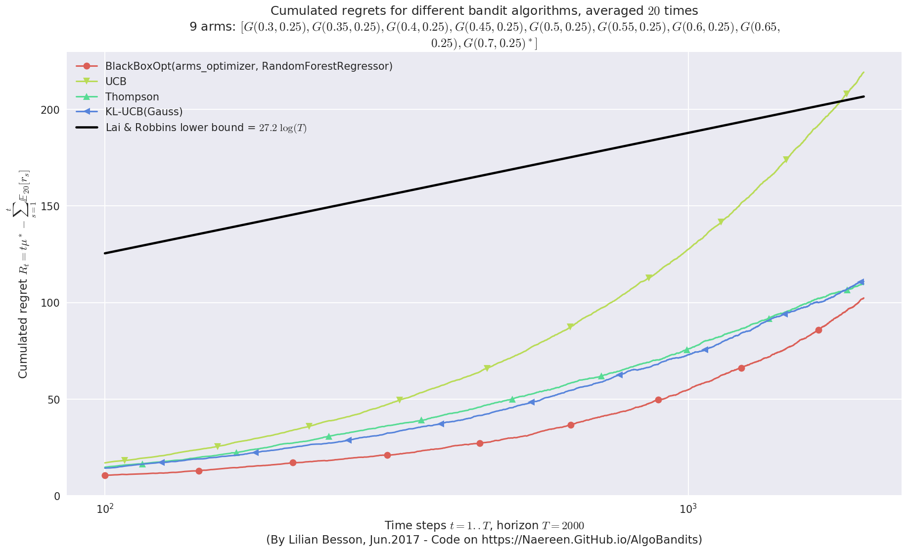
Non-logarithmic regret ?¶

But in terms of regret, it seems that the profile for BlackBoxOpt is not asymptotically logarithmic, contrarily to Thompson and klUCB (cf. see the first curve above, at the end on the right).

Note that the horizon is not that large, \(T = 2000\) is really not that very long.
And note that we didn’t try any other regressor (I tried them elsewhere: `ExtraTreesRegressor <https://scikit-optimize.github.io/learning/index.html#skopt.learning.ExtraTreesRegressor>`__ worked similarly but it is slower, and `GaussianProcessRegressor <https://scikit-optimize.github.io/learning/index.html#skopt.learning.GaussianProcessRegressor>`__ was failing, don’t really know why. I think it is not designed to work with Categorical inputs.

Comparing time complexity¶

Another aspect is the time complexity of the BlackBoxOpt policy. In the simulation above, we saw that it took way much time than the online bandit algorithms, like UCB, klUCB or Thompson sampling.

This notebook is here to illustrate my SMPyBandits library, for which a complete documentation is available, here at https://smpybandits.github.io/.

See the discussion on `skopt GitHub issues #407 <https://github.com/scikit-optimize/scikit-optimize/issues/407>`__.

That’s it for this demo! See you, folks!