Table of Contents
1 Easily creating MAB problems
1.1 Constant arms
1.2 Bernoulli arms
1.3 Gaussian arms
1.3.1 Wrong means for Gaussian arms ?
1.3.2 Closed form formula
1.3.3 With a larger variance ?
1.4 Exponential arms
1.5 Uniform arms
1.6 Arms with rewards outside of [0,1]
1.7 Gamma arms
1.8 Non-truncated Gaussian and Gamma arms
1.9 Conclusion
Easily creating MAB problems
First, be sure to be in the main folder, or to have installed `SMPyBandits <https://github.com/SMPyBandits/SMPyBandits>`__, and import MAB from Environment package:
[1]:
!pip install SMPyBandits watermark
%load_ext watermark
%watermark -v -m -p SMPyBandits -a "Lilian Besson"
Requirement already satisfied: SMPyBandits in ./venv3/lib/python3.6/site-packages (0.9.4)
Requirement already satisfied: watermark in ./venv3/lib/python3.6/site-packages (1.7.0)
Requirement already satisfied: scikit-learn in ./venv3/lib/python3.6/site-packages (from SMPyBandits) (0.20.0)
Requirement already satisfied: scikit-optimize in ./venv3/lib/python3.6/site-packages (from SMPyBandits) (0.5.2)
Requirement already satisfied: scipy>0.9 in ./venv3/lib/python3.6/site-packages (from SMPyBandits) (1.1.0)
Requirement already satisfied: numpy in ./venv3/lib/python3.6/site-packages (from SMPyBandits) (1.15.4)
Requirement already satisfied: matplotlib>=2 in ./venv3/lib/python3.6/site-packages (from SMPyBandits) (3.0.2)
Requirement already satisfied: seaborn in ./venv3/lib/python3.6/site-packages (from SMPyBandits) (0.9.0)
Requirement already satisfied: joblib in ./venv3/lib/python3.6/site-packages (from SMPyBandits) (0.13.0)
Requirement already satisfied: ipython in ./venv3/lib/python3.6/site-packages (from watermark) (7.1.1)
Requirement already satisfied: pyparsing!=2.0.4,!=2.1.2,!=2.1.6,>=2.0.1 in ./venv3/lib/python3.6/site-packages (from matplotlib>=2->SMPyBandits) (2.3.0)
Requirement already satisfied: kiwisolver>=1.0.1 in ./venv3/lib/python3.6/site-packages (from matplotlib>=2->SMPyBandits) (1.0.1)
Requirement already satisfied: python-dateutil>=2.1 in ./venv3/lib/python3.6/site-packages (from matplotlib>=2->SMPyBandits) (2.7.5)
Requirement already satisfied: cycler>=0.10 in ./venv3/lib/python3.6/site-packages (from matplotlib>=2->SMPyBandits) (0.10.0)
Requirement already satisfied: pandas>=0.15.2 in ./venv3/lib/python3.6/site-packages (from seaborn->SMPyBandits) (0.23.4)
Requirement already satisfied: setuptools>=18.5 in ./venv3/lib/python3.6/site-packages (from ipython->watermark) (40.6.2)
Requirement already satisfied: pexpect; sys_platform != "win32" in ./venv3/lib/python3.6/site-packages (from ipython->watermark) (4.6.0)
Requirement already satisfied: jedi>=0.10 in ./venv3/lib/python3.6/site-packages (from ipython->watermark) (0.13.1)
Requirement already satisfied: backcall in ./venv3/lib/python3.6/site-packages (from ipython->watermark) (0.1.0)
Requirement already satisfied: traitlets>=4.2 in ./venv3/lib/python3.6/site-packages (from ipython->watermark) (4.3.2)
Requirement already satisfied: pickleshare in ./venv3/lib/python3.6/site-packages (from ipython->watermark) (0.7.5)
Requirement already satisfied: pygments in ./venv3/lib/python3.6/site-packages (from ipython->watermark) (2.2.0)
Requirement already satisfied: prompt-toolkit<2.1.0,>=2.0.0 in ./venv3/lib/python3.6/site-packages (from ipython->watermark) (2.0.7)
Requirement already satisfied: decorator in ./venv3/lib/python3.6/site-packages (from ipython->watermark) (4.3.0)
Requirement already satisfied: six>=1.5 in ./venv3/lib/python3.6/site-packages (from python-dateutil>=2.1->matplotlib>=2->SMPyBandits) (1.11.0)
Requirement already satisfied: pytz>=2011k in ./venv3/lib/python3.6/site-packages (from pandas>=0.15.2->seaborn->SMPyBandits) (2018.7)
Requirement already satisfied: ptyprocess>=0.5 in ./venv3/lib/python3.6/site-packages (from pexpect; sys_platform != "win32"->ipython->watermark) (0.6.0)
Requirement already satisfied: parso>=0.3.0 in ./venv3/lib/python3.6/site-packages (from jedi>=0.10->ipython->watermark) (0.3.1)
Requirement already satisfied: ipython-genutils in ./venv3/lib/python3.6/site-packages (from traitlets>=4.2->ipython->watermark) (0.2.0)
Requirement already satisfied: wcwidth in ./venv3/lib/python3.6/site-packages (from prompt-toolkit<2.1.0,>=2.0.0->ipython->watermark) (0.1.7)
Info: Using the Jupyter notebook version of the tqdm() decorator, tqdm_notebook() ...
Lilian Besson

CPython 3.6.6
IPython 7.1.1

SMPyBandits 0.9.4

compiler   : GCC 8.0.1 20180414 (experimental) [trunk revision 259383
system     : Linux
release    : 4.15.0-38-generic
machine    : x86_64
processor  : x86_64
CPU cores  : 4
interpreter: 64bit
[2]:
from SMPyBandits.Environment import MAB
And also, import all the types of arms.
[3]:
from SMPyBandits.Arms import *
# Check it exists:
Constant, Bernoulli, Gaussian, Exponential, ExponentialFromMean, Poisson, UniformArm, Gamma, GammaFromMean
[3]:
(SMPyBandits.Arms.Constant.Constant,
 SMPyBandits.Arms.Bernoulli.Bernoulli,
 SMPyBandits.Arms.Gaussian.Gaussian,
 SMPyBandits.Arms.Exponential.Exponential,
 SMPyBandits.Arms.Exponential.ExponentialFromMean,
 SMPyBandits.Arms.Poisson.Poisson,
 SMPyBandits.Arms.UniformArm.UniformArm,
 SMPyBandits.Arms.Gamma.Gamma,
 SMPyBandits.Arms.Gamma.GammaFromMean)
[4]:
import matplotlib as mpl
mpl.rcParams['figure.figsize'] = (12.4, 7)
Constant arms
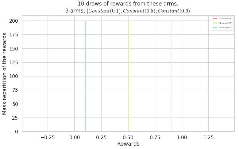
This is the simpler example of arms : rewards are constant, and not randomly drawn from a distribution. Let consider an example with \(K = 3\) arms.
[5]:
M_C = MAB([Constant(mu) for mu in [0.1, 0.5, 0.9]])
Creating a new MAB problem ...
  Taking arms of this MAB problem from a list of arms 'configuration' = [Constant(0.1), Constant(0.5), Constant(0.9)] ...
 - with 'arms' = [Constant(0.1), Constant(0.5), Constant(0.9)]
 - with 'means' = [0.1 0.5 0.9]
 - with 'nbArms' = 3
 - with 'maxArm' = 0.9
 - with 'minArm' = 0.1

This MAB problem has:
 - a [Lai & Robbins] complexity constant C(mu) = 2 ...
 - a Optimal Arm Identification factor H_OI(mu) = 26.67% ...
 - with 'arms' represented as: $[Constant(0.1), Constant(0.5), Constant(0.9)^*]$
The plotHistogram() method draws samples from each arm, and plot a histogram of their repartition. For constant arms, no need to take a lot of samples as they are constant.
[6]:
_ = M_C.plotHistogram(10)
Warning: forcing to use putatright = False because there is 3 items in the legend.
Bernoulli arms
Then it’s easy to create a Multi-Armed Bandit problem, instance of MAB class, either from a list of Arm objects:
[7]:
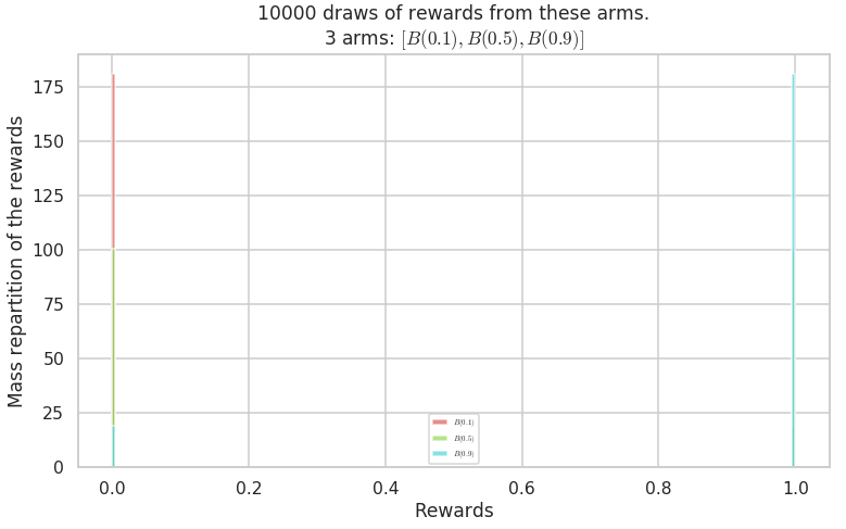
M_B = MAB([Bernoulli(mu) for mu in [0.1, 0.5, 0.9]])
Creating a new MAB problem ...
  Taking arms of this MAB problem from a list of arms 'configuration' = [B(0.1), B(0.5), B(0.9)] ...
 - with 'arms' = [B(0.1), B(0.5), B(0.9)]
 - with 'means' = [0.1 0.5 0.9]
 - with 'nbArms' = 3
 - with 'maxArm' = 0.9
 - with 'minArm' = 0.1

This MAB problem has:
 - a [Lai & Robbins] complexity constant C(mu) = 1.24 ...
 - a Optimal Arm Identification factor H_OI(mu) = 26.67% ...
 - with 'arms' represented as: $[B(0.1), B(0.5), B(0.9)^*]$
Or from a dictionary, with keys "arm_type" and "params":
[8]:
M_B = MAB({
    "arm_type": Bernoulli,
    "params": [0.1, 0.5, 0.9]
})
Creating a new MAB problem ...
  Reading arms of this MAB problem from a dictionnary 'configuration' = {'arm_type': <class 'SMPyBandits.Arms.Bernoulli.Bernoulli'>, 'params': [0.1, 0.5, 0.9]} ...
 - with 'arm_type' = <class 'SMPyBandits.Arms.Bernoulli.Bernoulli'>
 - with 'params' = [0.1, 0.5, 0.9]
 - with 'arms' = [B(0.1), B(0.5), B(0.9)]
 - with 'means' = [0.1 0.5 0.9]
 - with 'nbArms' = 3
 - with 'maxArm' = 0.9
 - with 'minArm' = 0.1

This MAB problem has:
 - a [Lai & Robbins] complexity constant C(mu) = 1.24 ...
 - a Optimal Arm Identification factor H_OI(mu) = 26.67% ...
 - with 'arms' represented as: $[B(0.1), B(0.5), B(0.9)^*]$
The plotHistogram() method draws a lot of samples from each arm, and plot a histogram of their repartition:
[9]:
_ = M_B.plotHistogram()
Warning: forcing to use putatright = False because there is 3 items in the legend.
Gaussian arms
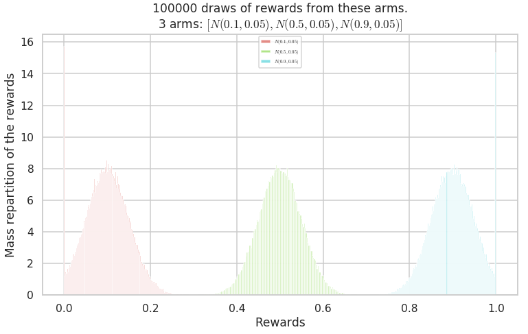
And with Gaussian arms, with a small variance of \(\sigma^2 = 0.05\), for rewards truncated into \([0, 1]\):
[10]:
M_G = MAB([Gaussian(mu, sigma=0.05) for mu in [0.1, 0.5, 0.9]])
Creating a new MAB problem ...
  Taking arms of this MAB problem from a list of arms 'configuration' = [N(0.1, 0.05), N(0.5, 0.05), N(0.9, 0.05)] ...
 - with 'arms' = [N(0.1, 0.05), N(0.5, 0.05), N(0.9, 0.05)]
 - with 'means' = [0.1 0.5 0.9]
 - with 'nbArms' = 3
 - with 'maxArm' = 0.9
 - with 'minArm' = 0.1

This MAB problem has:
 - a [Lai & Robbins] complexity constant C(mu) = 0.375 ...
 - a Optimal Arm Identification factor H_OI(mu) = 26.67% ...
 - with 'arms' represented as: $[N(0.1), N(0.5), N(0.9)^*], \sigma^2=0.05$
The histogram clearly shows that low-variance Gaussian arms are easy to separate:
[11]:
_ = M_G.plotHistogram(100000)
Warning: forcing to use putatright = False because there is 3 items in the legend.
Wrong means for Gaussian arms ?
The truncation seems to change the means.
For instance, the first arm (in red) has a small mass on the special value \(0\), so it probably reduces its mean.
Let’s estimate it empirically, and then check with the closed form solution.
[12]:
arm = Gaussian(0.1, sigma=0.05)
[13]:
mean = arm.mean
estimated_mean = np.mean(arm.draw_nparray((10000000,)))
[14]:
mean, estimated_mean
[14]:
(0.1, 0.10042691516597835)
[15]:
def relative_error(x, y):
    return abs(x - y) / x

relative_error(mean, estimated_mean)
[15]:
0.004269151659783421
\(\implies\) That’s a relative difference of \(0.4\%\), really negligible!
And for other values for \((\mu, \sigma)\):
[16]:
arm = Gaussian(0.7, sigma=3)
[17]:
mean = arm.mean
estimated_mean = np.mean(arm.draw_nparray((10000000,)))
[18]:
mean, estimated_mean
[18]:
(0.7, 0.5266068636711595)
[19]:
relative_error(mean, estimated_mean)
[19]:
0.2477044804697721
\(\implies\) That’s a relative difference of \(25\%\)!
Clearly, this effect cannot be neglected!
Closed form formula
Apparently, the closed form formula for the mean of a Gaussian arm \(\mathcal{N}(\mu, \sigma)\), truncated to :math:`[a,b]` is :
Let’s compute that.
[20]:
import numpy as np
from scipy.special import erf
The fonction
[21]:
def phi(xi):
    r"""The :math:`\phi(\xi)` function, defined by:

    .. math:: \phi(\xi) := \frac{1}{\sqrt{2 \pi}} \exp\left(- \frac12 \xi^2 \right)

    It is the probability density function of the standard normal distribution, see https://en.wikipedia.org/wiki/Standard_normal_distribution.
    """
    return np.exp(- 0.5 * xi**2) / np.sqrt(2. * np.pi)
The fonction
[22]:
def Phi(x):
    r"""The :math:`\Phi(x)` function, defined by:

    .. math:: \Phi(x) := \frac{1}{2} \left(1 + \mathrm{erf}\left( \frac{x}{\sqrt{2}} \right) \right).

    It is the probability density function of the standard normal distribution, see https://en.wikipedia.org/wiki/Cumulative_distribution_function
    """
    return (1. + erf(x / np.sqrt(2.))) / 2.
[23]:
mu, sigma, mini, maxi = arm.mu, arm.sigma, arm.min, arm.max
mu, sigma, mini, maxi
[23]:
(0.7, 3, 0, 1)
[24]:
other_mean = mu + sigma * (phi(mini) - phi(maxi)) / (Phi(maxi) - Phi(mini))
[25]:
mean, estimated_mean, other_mean
[25]:
(0.7, 0.5266068636711595, 2.0795866878592797)
Well, apparently, the theoretical formula is false for this case. It is not even bounded in \([0, 1]\)!
Let’s forget about this possible issue, and consider that the mean \(\mu\) of a Gaussian arm \(\mathcal{N}(\mu, \sigma)\) truncated to \([0,1]\) is indeed \(\mu\).
With a larger variance ?
But if the variance is larger, it can be very hard to differentiate between arms, and so MAB learning will be harder. With a big variance of \(\sigma^2 = 0.5\), for rewards truncated into \([0, 1]\):
[26]:
M_G = MAB([Gaussian(mu, sigma=0.10) for mu in [0.1, 0.5, 0.9]])
_ = M_G.plotHistogram(100000)
Creating a new MAB problem ...
  Taking arms of this MAB problem from a list of arms 'configuration' = [N(0.1, 0.1), N(0.5, 0.1), N(0.9, 0.1)] ...
 - with 'arms' = [N(0.1, 0.1), N(0.5, 0.1), N(0.9, 0.1)]
 - with 'means' = [0.1 0.5 0.9]
 - with 'nbArms' = 3
 - with 'maxArm' = 0.9
 - with 'minArm' = 0.1

This MAB problem has:
 - a [Lai & Robbins] complexity constant C(mu) = 0.75 ...
 - a Optimal Arm Identification factor H_OI(mu) = 26.67% ...
 - with 'arms' represented as: $[N(0.1), N(0.5), N(0.9)^*], \sigma^2=0.1$
Warning: forcing to use putatright = False because there is 3 items in the legend.
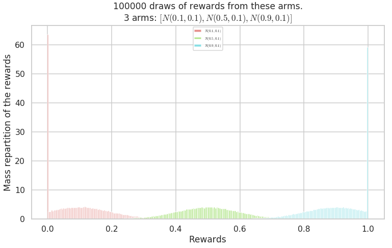
We see that due to the truncation, if mean of the Gaussian is too close to \(0\) or \(1\), then actual mean rewards is pushed to \(0\) or \(1\) (here the blue arm clearly has a mean higher than \(0.9\)).
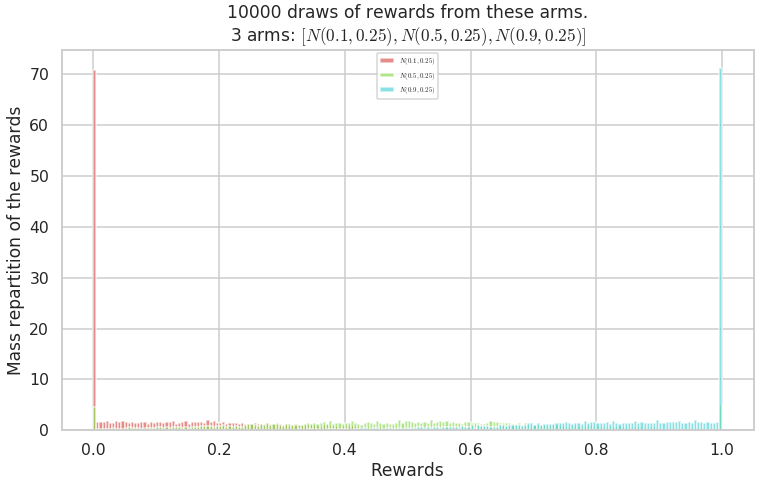
And for larger variances, it is even stronger:
[27]:
M_G = MAB([Gaussian(mu, sigma=0.25) for mu in [0.1, 0.5, 0.9]])
_ = M_G.plotHistogram()
Creating a new MAB problem ...
  Taking arms of this MAB problem from a list of arms 'configuration' = [N(0.1, 0.25), N(0.5, 0.25), N(0.9, 0.25)] ...
 - with 'arms' = [N(0.1, 0.25), N(0.5, 0.25), N(0.9, 0.25)]
 - with 'means' = [0.1 0.5 0.9]
 - with 'nbArms' = 3
 - with 'maxArm' = 0.9
 - with 'minArm' = 0.1

This MAB problem has:
 - a [Lai & Robbins] complexity constant C(mu) = 1.87 ...
 - a Optimal Arm Identification factor H_OI(mu) = 26.67% ...
 - with 'arms' represented as: $[N(0.1), N(0.5), N(0.9)^*], \sigma^2=0.25$
Warning: forcing to use putatright = False because there is 3 items in the legend.
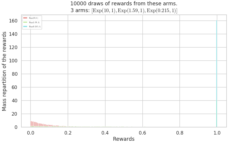
Exponential arms
We can do the same with (truncated) Exponential arms, and as a convenience I prefer to work with ExponentialFromMean, to use the mean and not the \(\lambda\) parameter to create the arm.
[28]:
M_E = MAB({ "arm_type": ExponentialFromMean, "params": [0.1, 0.5, 0.9]})
Creating a new MAB problem ...
  Reading arms of this MAB problem from a dictionnary 'configuration' = {'arm_type': <class 'SMPyBandits.Arms.Exponential.ExponentialFromMean'>, 'params': [0.1, 0.5, 0.9]} ...
 - with 'arm_type' = <class 'SMPyBandits.Arms.Exponential.ExponentialFromMean'>
 - with 'params' = [0.1, 0.5, 0.9]
 - with 'arms' = [\mathrm{Exp}(10, 1), \mathrm{Exp}(1.59, 1), \mathrm{Exp}(0.215, 1)]
 - with 'means' = [0.1 0.5 0.9]
 - with 'nbArms' = 3
 - with 'maxArm' = 0.9000000032329611
 - with 'minArm' = 0.10000000005466392

This MAB problem has:
 - a [Lai & Robbins] complexity constant C(mu) = 3.4 ...
 - a Optimal Arm Identification factor H_OI(mu) = 26.67% ...
 - with 'arms' represented as: $[\mathrm{Exp}(10, 1), \mathrm{Exp}(1.59, 1), \mathrm{Exp}(0.215, 1)^*]$
[29]:
_ = M_E.plotHistogram()
Warning: forcing to use putatright = False because there is 3 items in the legend.
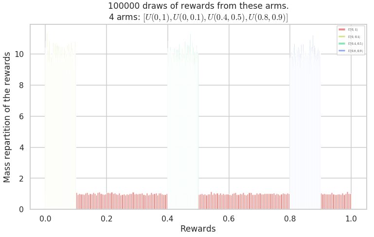
Uniform arms
Arms with rewards uniform in \([0,1]\), are continuous versions of Bernoulli\((0.5)\). They can also be uniform in other intervals.
[30]:
UniformArm(0, 1).lower_amplitude
UniformArm(0, 0.1).lower_amplitude
UniformArm(0.4, 0.5).lower_amplitude
UniformArm(0.8, 0.9).lower_amplitude
[30]:
(0, 1)
[30]:
(0, 0.1)
[30]:
(0.4, 0.09999999999999998)
[30]:
(0.8, 0.09999999999999998)
[31]:
M_U = MAB([UniformArm(0, 1), UniformArm(0, 0.1), UniformArm(0.4, 0.5), UniformArm(0.8, 0.9)])
Creating a new MAB problem ...
  Taking arms of this MAB problem from a list of arms 'configuration' = [U(0, 1), U(0, 0.1), U(0.4, 0.5), U(0.8, 0.9)] ...
 - with 'arms' = [U(0, 1), U(0, 0.1), U(0.4, 0.5), U(0.8, 0.9)]
 - with 'means' = [0.5  0.05 0.45 0.85]
 - with 'nbArms' = 4
 - with 'maxArm' = 0.8500000000000001
 - with 'minArm' = 0.05

This MAB problem has:
 - a [Lai & Robbins] complexity constant C(mu) = 2.47 ...
 - a Optimal Arm Identification factor H_OI(mu) = 36.25% ...
 - with 'arms' represented as: $[U(0, 1), U(0, 0.1), U(0.4, 0.5), U(0.8, 0.9)^*]$
[32]:
_ = M_U.plotHistogram(100000)
Warning: forcing to use putatright = False because there is 4 items in the legend.
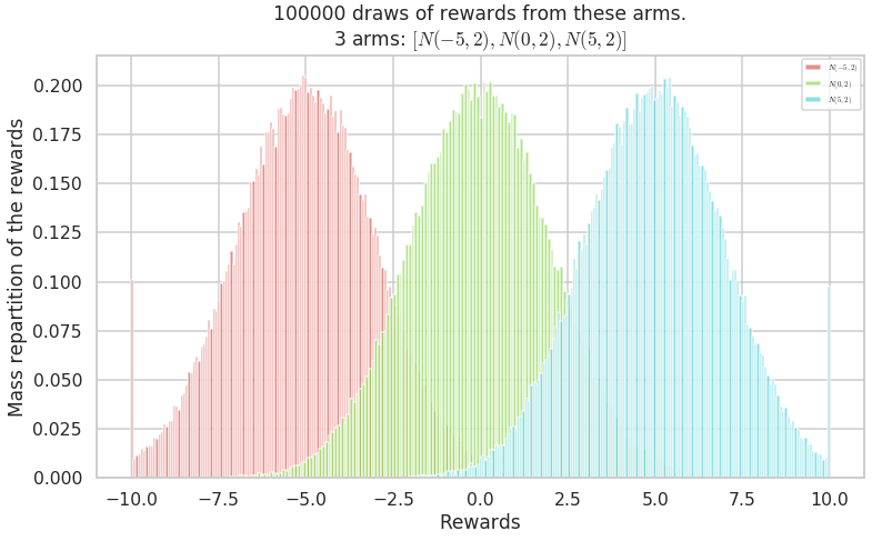
Arms with rewards outside of \([0, 1]\)
Of course, everything work similarly if rewards are not in \([0, 1]\) but in any interval \([a, b]\).
Note that all my algorithms assume \(a = \text{lower} = 0\) and \(b = 1\) (and use \(\text{amplitude} = b - a\) instead of \(b\)). They just need to be specified if we stop using the default choice \([0, 1]\).
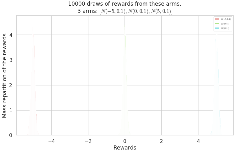
For example, Gaussian arms can be truncated into \([-10, 10]\) instead of \([0, 1]\). Let define some Gaussian arms, with means \(-5, 0, 5\) and a variance of \(\sigma^2 = 2\).
[33]:
M_G = MAB([Gaussian(mu, sigma=2, mini=-10, maxi=10) for mu in [-5, 0, 5]])
Creating a new MAB problem ...
  Taking arms of this MAB problem from a list of arms 'configuration' = [N(-5, 2), N(0, 2), N(5, 2)] ...
 - with 'arms' = [N(-5, 2), N(0, 2), N(5, 2)]
 - with 'means' = [-5  0  5]
 - with 'nbArms' = 3
 - with 'maxArm' = 5
 - with 'minArm' = -5

This MAB problem has:
 - a [Lai & Robbins] complexity constant C(mu) = 1.2 ...
 - a Optimal Arm Identification factor H_OI(mu) = 16.67% ...
 - with 'arms' represented as: $[N(-5), N(0), N(5)^*], \sigma^2=2$
[34]:
_ = M_G.plotHistogram(100000)
Warning: forcing to use putatright = False because there is 3 items in the legend.
[35]:
M_G = MAB([Gaussian(mu, sigma=0.1, mini=-10, maxi=10) for mu in [-5, 0, 5]])
Creating a new MAB problem ...
  Taking arms of this MAB problem from a list of arms 'configuration' = [N(-5, 0.1), N(0, 0.1), N(5, 0.1)] ...
 - with 'arms' = [N(-5, 0.1), N(0, 0.1), N(5, 0.1)]
 - with 'means' = [-5  0  5]
 - with 'nbArms' = 3
 - with 'maxArm' = 5
 - with 'minArm' = -5

This MAB problem has:
 - a [Lai & Robbins] complexity constant C(mu) = 0.06 ...
 - a Optimal Arm Identification factor H_OI(mu) = 16.67% ...
 - with 'arms' represented as: $[N(-5), N(0), N(5)^*], \sigma^2=0.1$
[36]:
_ = M_G.plotHistogram()
Warning: forcing to use putatright = False because there is 3 items in the legend.
Gamma arms
We can do the same with (truncated) Gamma arms, and as a convenience I prefer to work with GammaFromMean, to use the mean and not the \(k\) shape parameter to create the arm. The scale \(\theta\) is fixed to \(1\) by default, and here the rewards will be in \([0, 10]\).
[37]:
M_Gamma = MAB([GammaFromMean(shape, scale=1, mini=0, maxi=10) for shape in [1, 2, 3, 4, 5]])
Creating a new MAB problem ...
  Taking arms of this MAB problem from a list of arms 'configuration' = [\Gamma(1, 1), \Gamma(2, 1), \Gamma(3, 1), \Gamma(4, 1), \Gamma(5, 1)] ...
 - with 'arms' = [\Gamma(1, 1), \Gamma(2, 1), \Gamma(3, 1), \Gamma(4, 1), \Gamma(5, 1)]
 - with 'means' = [1. 2. 3. 4. 5.]
 - with 'nbArms' = 5
 - with 'maxArm' = 5.0
 - with 'minArm' = 1.0

This MAB problem has:
 - a [Lai & Robbins] complexity constant C(mu) = 75.7 ...
 - a Optimal Arm Identification factor H_OI(mu) = 60.00% ...
 - with 'arms' represented as: $[\Gamma(1, 1), \Gamma(2, 1), \Gamma(3, 1), \Gamma(4, 1), \Gamma(5, 1)^*]$
[38]:
_ = M_Gamma.plotHistogram(100000)
Warning: forcing to use putatright = False because there is 5 items in the legend.
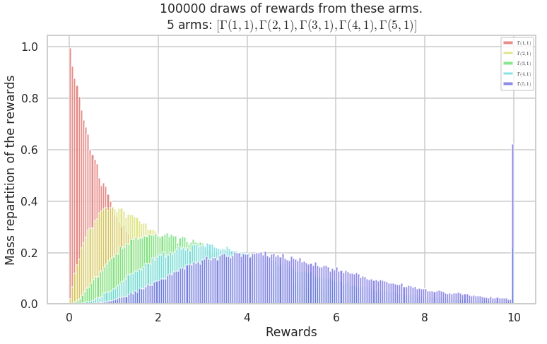
As for Gaussian arms, the truncation is strongly changing the means of the arm rewards. Here the arm with mean parameter \(5\) has an empirical mean close to \(10\) due to truncation.
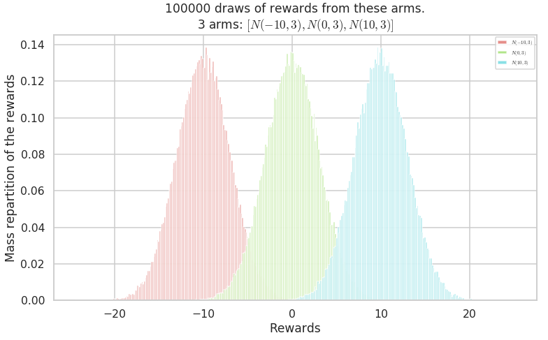
Non-truncated Gaussian and Gamma arms
Let try with non-truncated rewards.
[39]:
M_G = MAB([Gaussian(mu, sigma=3, mini=float('-inf'), maxi=float('+inf')) for mu in [-10, 0, 10]])
Creating a new MAB problem ...
  Taking arms of this MAB problem from a list of arms 'configuration' = [N(-10, 3), N(0, 3), N(10, 3)] ...
 - with 'arms' = [N(-10, 3), N(0, 3), N(10, 3)]
 - with 'means' = [-10   0  10]
 - with 'nbArms' = 3
 - with 'maxArm' = 10
 - with 'minArm' = -10

This MAB problem has:
 - a [Lai & Robbins] complexity constant C(mu) = 0.9 ...
 - a Optimal Arm Identification factor H_OI(mu) = 66.67% ...
 - with 'arms' represented as: $[N(-10), N(0), N(10)^*], \sigma^2=3$
[40]:
_ = M_G.plotHistogram(100000)
Warning: forcing to use putatright = False because there is 3 items in the legend.
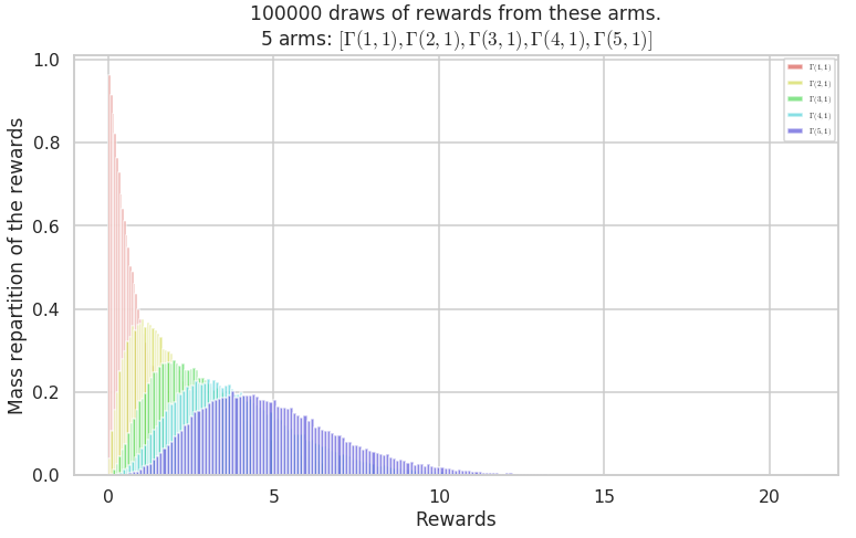
And with non-truncated Gamma arms ?
[41]:
M_Gamma = MAB([GammaFromMean(shape, scale=1, mini=float('-inf'), maxi=float('+inf')) for shape in [1, 2, 3, 4, 5]])
_ = M_Gamma.plotHistogram(100000)
Creating a new MAB problem ...
  Taking arms of this MAB problem from a list of arms 'configuration' = [\Gamma(1, 1), \Gamma(2, 1), \Gamma(3, 1), \Gamma(4, 1), \Gamma(5, 1)] ...
 - with 'arms' = [\Gamma(1, 1), \Gamma(2, 1), \Gamma(3, 1), \Gamma(4, 1), \Gamma(5, 1)]
 - with 'means' = [1. 2. 3. 4. 5.]
 - with 'nbArms' = 5
 - with 'maxArm' = 5.0
 - with 'minArm' = 1.0

This MAB problem has:
 - a [Lai & Robbins] complexity constant C(mu) = 75.7 ...
 - a Optimal Arm Identification factor H_OI(mu) = 80.00% ...
 - with 'arms' represented as: $[\Gamma(1, 1), \Gamma(2, 1), \Gamma(3, 1), \Gamma(4, 1), \Gamma(5, 1)^*]$
Warning: forcing to use putatright = False because there is 5 items in the legend.
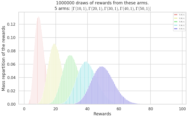
[42]:
M_Gamma = MAB([GammaFromMean(shape, scale=1, mini=float('-inf'), maxi=float('+inf')) for shape in [10, 20, 30, 40, 50]])
_ = M_Gamma.plotHistogram(1000000)
Creating a new MAB problem ...
  Taking arms of this MAB problem from a list of arms 'configuration' = [\Gamma(10, 1), \Gamma(20, 1), \Gamma(30, 1), \Gamma(40, 1), \Gamma(50, 1)] ...
 - with 'arms' = [\Gamma(10, 1), \Gamma(20, 1), \Gamma(30, 1), \Gamma(40, 1), \Gamma(50, 1)]
 - with 'means' = [10. 20. 30. 40. 50.]
 - with 'nbArms' = 5
 - with 'maxArm' = 50.0
 - with 'minArm' = 10.0

This MAB problem has:
 - a [Lai & Robbins] complexity constant C(mu) = 757 ...
 - a Optimal Arm Identification factor H_OI(mu) = 80.00% ...
 - with 'arms' represented as: $[\Gamma(10, 1), \Gamma(20, 1), \Gamma(30, 1), \Gamma(40, 1), \Gamma(50, 1)^*]$
Warning: forcing to use putatright = False because there is 5 items in the legend.
Conclusion
This small notebook demonstrated how to define arms and Multi-Armed Bandit problems in my framework, SMPyBandits.