Table of Contents
1 Requirements and helper functions
1.1 Requirements
1.2 Mathematical notations for stationary problems
1.3 Generating stationary data
1.4 Mathematical notations for piecewise stationary problems
1.5 Generating fake piecewise stationary data
2 Python implementations of some statistical tests
2.1 Monitored
2.2 CUSUM
2.3 PHT
2.4 Gaussian GLR
2.5 Bernoulli GLR
2.6 Sub-Gaussian GLR
2.7 List of all Python algorithms
3 Comparing the different implementations
3.1 Generating some toy data
3.2 Checking time efficiency
3.3 Checking detection delay
3.4 Checking false alarm probabilities
3.5 Checking missed detection probabilities
4 More simulations and some plots
4.1 Run a check for a grid of values
4.2 A version using joblib.Parallel to use multi-core computations
4.3 Checking on a small grid of values
4.4 Plotting the result as a 2D image
4.4.1 First example
4.4.1.1 For Monitored
4.4.1.2 For CUSUM
4.4.2 Second example
4.4.2.1 For Monitored
4.4.2.2 For Monitored for Gaussian data
4.4.2.3 For CUSUM
4.4.2.4 For PHT
4.4.2.5 For Bernoulli GLR
4.4.2.6 For Gaussian GLR
4.4.2.7 For Sub-Gaussian GLR
5 Exploring the parameters of change point detection algorithms: how to tune them?
5.1 A simple problem function
5.2 A generic function
5.3 Plotting the result as a 1D plot
5.4 Experiments for Monitored
5.5 Experiments for Bernoulli GLR
5.6 Experiments for Gaussian GLR
5.7 Experiments for CUSUM
5.8 Experiments for Sub-Gaussian GLR
5.9 Other experiments
6 Conclusions
Requirements and helper functions
Requirements
This notebook requires to have `numpy <https://www.numpy.org/>`__ and `matplotlib <https://matplotlib.org/>`__ installed. One function needs a function from `scipy.special <https://docs.scipy.org/doc/scipy/reference/generated/scipy.special.comb.html#scipy.special.comb>`__. `joblib <https://joblib.readthedocs.io/en/latest/>`__ is used to have parallel computations (at the end).
The bottleneck performance of the main functions are very simple functions, for which we can write efficient versions using either `numba.jit <https://numba.pydata.org/numba-doc/latest/reference/jit-compilation.html#numba.jit>`__ or `cython <https://cython.readthedocs.io/en/latest/src/quickstart/build.html#jupyter-notebook>`__.
[3]:
!pip3 install watermark numpy scipy matplotlib joblib numba cython
%load_ext watermark
%watermark -v -m -p numpy,scipy,matplotlib,joblib,numba,cython -a "Lilian Besson and Emilie Kaufmann"
Requirement already satisfied: watermark in /usr/local/lib/python3.6/dist-packages (1.5.0)
Requirement already satisfied: numpy in /usr/local/lib/python3.6/dist-packages (1.15.4)
Requirement already satisfied: scipy in /usr/local/lib/python3.6/dist-packages (1.1.0)
Requirement already satisfied: matplotlib in /usr/local/lib/python3.6/dist-packages (3.0.2)
Requirement already satisfied: joblib in /usr/local/lib/python3.6/dist-packages (0.12.1)
Requirement already satisfied: numba in /usr/local/lib/python3.6/dist-packages (0.41.0)
Requirement already satisfied: cython in /usr/local/lib/python3.6/dist-packages (0.29.1)
Requirement already satisfied: ipython in /usr/local/lib/python3.6/dist-packages (from watermark) (7.2.0)
Requirement already satisfied: cycler>=0.10 in /usr/local/lib/python3.6/dist-packages (from matplotlib) (0.10.0)
Requirement already satisfied: kiwisolver>=1.0.1 in /usr/local/lib/python3.6/dist-packages (from matplotlib) (1.0.1)
Requirement already satisfied: pyparsing!=2.0.4,!=2.1.2,!=2.1.6,>=2.0.1 in /usr/local/lib/python3.6/dist-packages (from matplotlib) (2.3.0)
Requirement already satisfied: python-dateutil>=2.1 in /usr/local/lib/python3.6/dist-packages (from matplotlib) (2.7.3)
Requirement already satisfied: llvmlite>=0.26.0dev0 in /usr/local/lib/python3.6/dist-packages (from numba) (0.26.0)
Requirement already satisfied: prompt-toolkit<2.1.0,>=2.0.0 in /usr/local/lib/python3.6/dist-packages (from ipython->watermark) (2.0.7)
Requirement already satisfied: jedi>=0.10 in /usr/local/lib/python3.6/dist-packages (from ipython->watermark) (0.12.1)
Requirement already satisfied: pygments in /usr/local/lib/python3.6/dist-packages (from ipython->watermark) (2.2.0)
Requirement already satisfied: decorator in /usr/local/lib/python3.6/dist-packages (from ipython->watermark) (4.3.0)
Requirement already satisfied: setuptools>=18.5 in /usr/local/lib/python3.6/dist-packages (from ipython->watermark) (40.5.0)
Requirement already satisfied: traitlets>=4.2 in /usr/local/lib/python3.6/dist-packages (from ipython->watermark) (4.3.2)
Requirement already satisfied: pickleshare in /usr/local/lib/python3.6/dist-packages (from ipython->watermark) (0.7.5)
Requirement already satisfied: pexpect; sys_platform != "win32" in /usr/local/lib/python3.6/dist-packages (from ipython->watermark) (4.6.0)
Requirement already satisfied: backcall in /usr/local/lib/python3.6/dist-packages (from ipython->watermark) (0.1.0)
Requirement already satisfied: six in /home/lilian/.local/lib/python3.6/site-packages (from cycler>=0.10->matplotlib) (1.11.0)
Requirement already satisfied: wcwidth in /usr/local/lib/python3.6/dist-packages (from prompt-toolkit<2.1.0,>=2.0.0->ipython->watermark) (0.1.7)
Requirement already satisfied: parso>=0.3.0 in /usr/local/lib/python3.6/dist-packages (from jedi>=0.10->ipython->watermark) (0.3.1)
Requirement already satisfied: ipython-genutils in /usr/local/lib/python3.6/dist-packages (from traitlets>=4.2->ipython->watermark) (0.2.0)
Requirement already satisfied: ptyprocess>=0.5 in /usr/local/lib/python3.6/dist-packages (from pexpect; sys_platform != "win32"->ipython->watermark) (0.6.0)
The watermark extension is already loaded. To reload it, use:
  %reload_ext watermark
Lilian Besson and Emilie Kaufmann

CPython 3.6.7
IPython 7.2.0

numpy 1.15.4
scipy 1.1.0
matplotlib 3.0.2
joblib 0.12.1
numba 0.41.0
cython 0.29.1

compiler   : GCC 8.2.0
system     : Linux
release    : 4.15.0-42-generic
machine    : x86_64
processor  : x86_64
CPU cores  : 4
interpreter: 64bit
[4]:
import numpy as np
[5]:
try:
    from tqdm import tqdm_notebook as tqdm
except:
    def tqdm(iterator, *args, **kwargs):
        return iterator
Mathematical notations for stationary problems
We consider \(K \geq 1\) arms, which are distributions \(\nu_k\). We focus on Bernoulli distributions, which are characterized by their means, \(\nu_k = \mathcal{B}(\mu_k)\) for \(\mu_k\in[0,1]\). A stationary bandit problem is defined here by the vector \([\mu_1,\dots,\mu_K]\).
For a fixed problem and a horizon \(T\in\mathbb{N}\), \(T\geq1\), we draw samples from the \(K\) distributions to get data: \(\forall t, r_k(t) \sim \nu_k\), ie, \(\mathbb{P}(r_k(t) = 1) = \mu_k\) and \(r_k(t) \in \{0,1\}\).
Generating stationary data
Here we give some examples of stationary problems and examples of data we can draw from them.
[13]:
def bernoulli_samples(means, horizon=1000):
    if np.size(means) == 1:
        return np.random.binomial(1, means, size=horizon)
    else:
        results = np.zeros((np.size(means), horizon))
        for i, mean in enumerate(means):
            results[i] = np.random.binomial(1, mean, size=horizon)
        return results
[14]:
problem1 = [0.5]

bernoulli_samples(problem1, horizon=20)
[14]:
array([0, 1, 1, 0, 1, 0, 1, 0, 1, 0, 0, 0, 1, 0, 1, 1, 0, 0, 0, 0])
[27]:
%timeit bernoulli_samples(problem1, horizon=1000)
61.5 µs ± 2.59 µs per loop (mean ± std. dev. of 7 runs, 10000 loops each)
Now for Gaussian data:
[49]:
sigma = 0.25 # Bernoulli are 1/4-sub Gaussian too!
[50]:
def gaussian_samples(means, horizon=1000, sigma=sigma):
    if np.size(means) == 1:
        return np.random.normal(loc=means, scale=sigma, size=horizon)
    else:
        results = np.zeros((np.size(means), horizon))
        for i, mean in enumerate(means):
            results[i] = np.random.normal(loc=mean, scale=sigma, size=horizon)
        return results
[51]:
gaussian_samples(problem1, horizon=20)
[51]:
array([ 0.62387502,  0.25629644,  0.67019174,  0.17045626,  0.64599757,
        0.37851622,  0.7365035 ,  0.59688851,  0.63485378,  0.59576263,
        0.27670489,  0.69860233,  0.49817269,  0.26672791, -0.05480486,
        0.43916024,  0.4352945 ,  0.630749  , -0.11451167,  0.11158323])
[52]:
%timeit gaussian_samples(problem1, horizon=1000)
75.8 µs ± 4.3 µs per loop (mean ± std. dev. of 7 runs, 10000 loops each)
For bandit problem with \(K \geq 2\) arms, the goal is to design an online learning algorithm that roughly do the following:
For time \(t=1\) to \(t=T\) (unknown horizon)
Algorithm \(A\) decide to draw arm \(A(t) \in\{1,\dots,K\}\),
Get the reward \(r(t) = r_{A(t)}(t) \sim \nu_{A(t)}\) from the (Bernoulli) distribution of that arm,
Give this observation of reward \(r(t)\) coming from arm \(A(t)\) to the algorithm,
Update internal state of the algorithm
An algorithm is efficient if it obtains a high (expected) sum reward, ie, \(\sum_{t=1}^T r(t)\).
Note that I don’t focus on bandit algorithm here.
[9]:
problem2 = [0.1, 0.5, 0.9]

bernoulli_samples(problem2, horizon=20)
[9]:
array([[0., 0., 0., 0., 0., 0., 0., 0., 0., 1., 0., 0., 0., 0., 0., 0.,
        0., 0., 0., 0.],
       [1., 1., 0., 1., 0., 0., 1., 0., 1., 0., 1., 1., 1., 0., 0., 1.,
        0., 0., 1., 0.],
       [1., 0., 1., 1., 1., 0., 1., 1., 1., 1., 1., 1., 1., 1., 1., 1.,
        0., 1., 1., 1.]])
[10]:
problem2 = [0.1, 0.5, 0.9]

gaussian_samples(problem2, horizon=20)
[10]:
array([[ 0.46905853,  0.08312363, -0.23166553,  0.59750825,  0.23356612,
        -0.02132874, -0.26851831,  0.18202564,  0.37409142, -0.14397223,
        -0.22241626, -0.18888125, -0.13127815,  0.2314255 ,  0.49433066,
         0.39645143, -0.11529154, -0.13321403,  0.34457873, -0.16463127],
       [ 0.09801182,  0.8898005 ,  0.76216447,  0.72837837,  0.25624864,
         0.71225959,  0.56964125,  0.6309913 ,  1.06315774,  0.28064027,
         0.2251329 ,  0.61036472,  0.43995415,  0.57338936,  0.74570767,
         0.89390964,  0.50845914,  0.62240528,  0.27255829,  0.03454648],
       [ 1.04280525,  0.38307288,  0.81820526,  0.95947436,  1.21587846,
         0.82568302,  0.60475185,  1.09188758,  1.40998237,  0.7291101 ,
         0.94030203,  0.95715236,  0.6893489 ,  1.26446965,  0.80080259,
         0.96966515,  0.79117913,  0.48041062,  0.92280092,  1.27883349]])
For instance on these data, the best arm is clearly the third one, with expected reward of \(\mu^* = \max_k \mu_k = 0.9\).
Mathematical notations for piecewise stationary problems
Now we fix the horizon \(T\in\mathbb{N}\), \(T\geq1\) and we also consider a set of \(\Upsilon_T\) break points, \(\tau_1,\dots,\tau_{\Upsilon_T} \in\{1,\dots,T\}\). We denote \(\tau_0 = 0\) and \(\tau_{\Upsilon_T+1} = T\) for convenience of notations. We can assume that breakpoints are far “enough” from each other, for instance that there exists an integer \(N\in\mathbb{N},N\geq1\) such that \(\min_{i=0}^{\Upsilon_T} \tau_{i+1} - \tau_i \geq N K\). That is, on each stationary interval, a uniform sampling of the \(K\) arms gives at least \(N\) samples by arm.
Now, in any stationary interval \([\tau_i + 1, \tau_{i+1}]\), the \(K \geq 1\) arms are distributions \(\nu_k^{(i)}\). We focus on Bernoulli distributions, which are characterized by their means, \(\nu_k^{(i)} := \mathcal{B}(\mu_k^{(i)})\) for \(\mu_k^{(i)}\in[0,1]\). A piecewise stationary bandit problem is defined here by the vector \([\mu_k^{(i)}]_{1\leq k \leq K, 1 \leq i \leq \Upsilon_T}\).
For a fixed problem and a horizon \(T\in\mathbb{N}\), \(T\geq1\), we draw samples from the \(K\) distributions to get data: \(\forall t, r_k(t) \sim \nu_k^{(i)}\) for \(i\) the unique index of stationary interval such that \(t\in[\tau_i + 1, \tau_{i+1}]\).
Generating fake piecewise stationary data
The format to define piecewise stationary problem will be the following. It is compact but generic!
The first example considers a unique arm, with 2 breakpoints uniformly spaced. - On the first interval, for instance from \(t=1\) to \(t=500\), that is \(\tau_1 = 500\), \(\mu_1^{(1)} = 0.1\), - On the second interval, for instance from \(t=501\) to \(t=1000\), that is \(\tau_2 = 100\), \(\mu_1^{(2)} = 0.5\), - On the third interval, for instance from \(t=1001\) to \(t=1500\), that \(\mu_1^{(3)} = 0.9\).
[53]:
# With 1 arm only!
problem_piecewise_0 = lambda horizon: {
    "listOfMeans": [
        [0.1],  # 0    to 499
        [0.5],  # 500  to 999
        [0.8],  # 1000  to 1499
    ],
    "changePoints": [
        int(0    * horizon / 1500.0),
        int(500  * horizon / 1500.0),
        int(1000  * horizon / 1500.0),
    ],
}
[54]:
# With 2 arms
problem_piecewise_1 = lambda horizon: {
    "listOfMeans": [
        [0.1, 0.2],  # 0    to 399
        [0.1, 0.3],  # 400  to 799
        [0.5, 0.3],  # 800  to 1199
        [0.4, 0.3],  # 1200 to 1599
        [0.3, 0.9],  # 1600 to end
    ],
    "changePoints": [
        int(0    * horizon / 2000.0),
        int(400  * horizon / 2000.0),
        int(800  * horizon / 2000.0),
        int(1200 * horizon / 2000.0),
        int(1600 * horizon / 2000.0),
    ],
}
[55]:
# With 3 arms
problem_piecewise_2 = lambda horizon: {
    "listOfMeans": [
        [0.2, 0.5, 0.9],  # 0    to 399
        [0.2, 0.2, 0.9],  # 400  to 799
        [0.2, 0.2, 0.1],  # 800  to 1199
        [0.7, 0.2, 0.1],  # 1200 to 1599
        [0.7, 0.5, 0.1],  # 1600 to end
    ],
    "changePoints": [
        int(0    * horizon / 2000.0),
        int(400  * horizon / 2000.0),
        int(800  * horizon / 2000.0),
        int(1200 * horizon / 2000.0),
        int(1600 * horizon / 2000.0),
    ],
}
[56]:
# With 3 arms
problem_piecewise_3 = lambda horizon: {
    "listOfMeans": [
        [0.4, 0.5, 0.9],  # 0    to 399
        [0.5, 0.4, 0.7],  # 400  to 799
        [0.6, 0.3, 0.5],  # 800  to 1199
        [0.7, 0.2, 0.3],  # 1200 to 1599
        [0.8, 0.1, 0.1],  # 1600 to end
    ],
    "changePoints": [
        int(0    * horizon / 2000.0),
        int(400  * horizon / 2000.0),
        int(800  * horizon / 2000.0),
        int(1200 * horizon / 2000.0),
        int(1600 * horizon / 2000.0),
    ],
}
Now we can write a utility function that transform this compact representation into a full list of means.
[57]:
def getFullHistoryOfMeans(problem, horizon=2000):
    """Return the vector of mean of the arms, for a piece-wise stationary MAB.

    - It is a numpy array of shape (nbArms, horizon).
    """
    pb = problem(horizon)
    listOfMeans, changePoints = pb['listOfMeans'], pb['changePoints']
    nbArms = len(listOfMeans[0])
    if horizon is None:
        horizon = np.max(changePoints)
    meansOfArms = np.ones((nbArms, horizon))
    for armId in range(nbArms):
        nbChangePoint = 0
        for t in range(horizon):
            if nbChangePoint < len(changePoints) - 1 and t >= changePoints[nbChangePoint + 1]:
                nbChangePoint += 1
            meansOfArms[armId][t] = listOfMeans[nbChangePoint][armId]
    return meansOfArms
For examples :
[16]:
getFullHistoryOfMeans(problem_piecewise_0, horizon=50)
[16]:
array([[0.1, 0.1, 0.1, 0.1, 0.1, 0.1, 0.1, 0.1, 0.1, 0.1, 0.1, 0.1, 0.1,
        0.1, 0.1, 0.1, 0.5, 0.5, 0.5, 0.5, 0.5, 0.5, 0.5, 0.5, 0.5, 0.5,
        0.5, 0.5, 0.5, 0.5, 0.5, 0.5, 0.5, 0.8, 0.8, 0.8, 0.8, 0.8, 0.8,
        0.8, 0.8, 0.8, 0.8, 0.8, 0.8, 0.8, 0.8, 0.8, 0.8, 0.8]])
[17]:
getFullHistoryOfMeans(problem_piecewise_1, horizon=50)
[17]:
array([[0.1, 0.1, 0.1, 0.1, 0.1, 0.1, 0.1, 0.1, 0.1, 0.1, 0.1, 0.1, 0.1,
        0.1, 0.1, 0.1, 0.1, 0.1, 0.1, 0.1, 0.5, 0.5, 0.5, 0.5, 0.5, 0.5,
        0.5, 0.5, 0.5, 0.5, 0.4, 0.4, 0.4, 0.4, 0.4, 0.4, 0.4, 0.4, 0.4,
        0.4, 0.3, 0.3, 0.3, 0.3, 0.3, 0.3, 0.3, 0.3, 0.3, 0.3],
       [0.2, 0.2, 0.2, 0.2, 0.2, 0.2, 0.2, 0.2, 0.2, 0.2, 0.3, 0.3, 0.3,
        0.3, 0.3, 0.3, 0.3, 0.3, 0.3, 0.3, 0.3, 0.3, 0.3, 0.3, 0.3, 0.3,
        0.3, 0.3, 0.3, 0.3, 0.3, 0.3, 0.3, 0.3, 0.3, 0.3, 0.3, 0.3, 0.3,
        0.3, 0.9, 0.9, 0.9, 0.9, 0.9, 0.9, 0.9, 0.9, 0.9, 0.9]])
[18]:
getFullHistoryOfMeans(problem_piecewise_2, horizon=50)
[18]:
array([[0.2, 0.2, 0.2, 0.2, 0.2, 0.2, 0.2, 0.2, 0.2, 0.2, 0.2, 0.2, 0.2,
        0.2, 0.2, 0.2, 0.2, 0.2, 0.2, 0.2, 0.2, 0.2, 0.2, 0.2, 0.2, 0.2,
        0.2, 0.2, 0.2, 0.2, 0.7, 0.7, 0.7, 0.7, 0.7, 0.7, 0.7, 0.7, 0.7,
        0.7, 0.7, 0.7, 0.7, 0.7, 0.7, 0.7, 0.7, 0.7, 0.7, 0.7],
       [0.5, 0.5, 0.5, 0.5, 0.5, 0.5, 0.5, 0.5, 0.5, 0.5, 0.2, 0.2, 0.2,
        0.2, 0.2, 0.2, 0.2, 0.2, 0.2, 0.2, 0.2, 0.2, 0.2, 0.2, 0.2, 0.2,
        0.2, 0.2, 0.2, 0.2, 0.2, 0.2, 0.2, 0.2, 0.2, 0.2, 0.2, 0.2, 0.2,
        0.2, 0.5, 0.5, 0.5, 0.5, 0.5, 0.5, 0.5, 0.5, 0.5, 0.5],
       [0.9, 0.9, 0.9, 0.9, 0.9, 0.9, 0.9, 0.9, 0.9, 0.9, 0.9, 0.9, 0.9,
        0.9, 0.9, 0.9, 0.9, 0.9, 0.9, 0.9, 0.1, 0.1, 0.1, 0.1, 0.1, 0.1,
        0.1, 0.1, 0.1, 0.1, 0.1, 0.1, 0.1, 0.1, 0.1, 0.1, 0.1, 0.1, 0.1,
        0.1, 0.1, 0.1, 0.1, 0.1, 0.1, 0.1, 0.1, 0.1, 0.1, 0.1]])
[19]:
getFullHistoryOfMeans(problem_piecewise_3, horizon=50)
[19]:
array([[0.4, 0.4, 0.4, 0.4, 0.4, 0.4, 0.4, 0.4, 0.4, 0.4, 0.5, 0.5, 0.5,
        0.5, 0.5, 0.5, 0.5, 0.5, 0.5, 0.5, 0.6, 0.6, 0.6, 0.6, 0.6, 0.6,
        0.6, 0.6, 0.6, 0.6, 0.7, 0.7, 0.7, 0.7, 0.7, 0.7, 0.7, 0.7, 0.7,
        0.7, 0.8, 0.8, 0.8, 0.8, 0.8, 0.8, 0.8, 0.8, 0.8, 0.8],
       [0.5, 0.5, 0.5, 0.5, 0.5, 0.5, 0.5, 0.5, 0.5, 0.5, 0.4, 0.4, 0.4,
        0.4, 0.4, 0.4, 0.4, 0.4, 0.4, 0.4, 0.3, 0.3, 0.3, 0.3, 0.3, 0.3,
        0.3, 0.3, 0.3, 0.3, 0.2, 0.2, 0.2, 0.2, 0.2, 0.2, 0.2, 0.2, 0.2,
        0.2, 0.1, 0.1, 0.1, 0.1, 0.1, 0.1, 0.1, 0.1, 0.1, 0.1],
       [0.9, 0.9, 0.9, 0.9, 0.9, 0.9, 0.9, 0.9, 0.9, 0.9, 0.7, 0.7, 0.7,
        0.7, 0.7, 0.7, 0.7, 0.7, 0.7, 0.7, 0.5, 0.5, 0.5, 0.5, 0.5, 0.5,
        0.5, 0.5, 0.5, 0.5, 0.3, 0.3, 0.3, 0.3, 0.3, 0.3, 0.3, 0.3, 0.3,
        0.3, 0.1, 0.1, 0.1, 0.1, 0.1, 0.1, 0.1, 0.1, 0.1, 0.1]])
And now we need to be able to generate samples from such distributions.
[58]:
def piecewise_bernoulli_samples(problem, horizon=1000):
    fullMeans = getFullHistoryOfMeans(problem, horizon=horizon)
    nbArms, horizon = np.shape(fullMeans)
    results = np.zeros((nbArms, horizon))
    for i in range(nbArms):
        mean_i = fullMeans[i, :]
        for t in range(horizon):
            mean_i_t = max(0, min(1, mean_i[t]))  # crop to [0, 1] !
            results[i, t] = np.random.binomial(1, mean_i_t)
    return results
[59]:
def piecewise_gaussian_samples(problem, horizon=1000, sigma=sigma):
    fullMeans = getFullHistoryOfMeans(problem, horizon=horizon)
    nbArms, horizon = np.shape(fullMeans)
    results = np.zeros((nbArms, horizon))
    for i in range(nbArms):
        mean_i = fullMeans[i, :]
        for t in range(horizon):
            mean_i_t = mean_i[t]
            results[i, t] = np.random.normal(loc=mean_i_t, scale=sigma, size=1)
    return results
Examples:
[22]:
getFullHistoryOfMeans(problem_piecewise_0, horizon=100)
piecewise_bernoulli_samples(problem_piecewise_0, horizon=100)
[22]:
array([[0.1, 0.1, 0.1, 0.1, 0.1, 0.1, 0.1, 0.1, 0.1, 0.1, 0.1, 0.1, 0.1,
        0.1, 0.1, 0.1, 0.1, 0.1, 0.1, 0.1, 0.1, 0.1, 0.1, 0.1, 0.1, 0.1,
        0.1, 0.1, 0.1, 0.1, 0.1, 0.1, 0.1, 0.5, 0.5, 0.5, 0.5, 0.5, 0.5,
        0.5, 0.5, 0.5, 0.5, 0.5, 0.5, 0.5, 0.5, 0.5, 0.5, 0.5, 0.5, 0.5,
        0.5, 0.5, 0.5, 0.5, 0.5, 0.5, 0.5, 0.5, 0.5, 0.5, 0.5, 0.5, 0.5,
        0.5, 0.8, 0.8, 0.8, 0.8, 0.8, 0.8, 0.8, 0.8, 0.8, 0.8, 0.8, 0.8,
        0.8, 0.8, 0.8, 0.8, 0.8, 0.8, 0.8, 0.8, 0.8, 0.8, 0.8, 0.8, 0.8,
        0.8, 0.8, 0.8, 0.8, 0.8, 0.8, 0.8, 0.8, 0.8]])
[22]:
array([[0., 1., 0., 1., 0., 1., 1., 0., 0., 0., 1., 0., 0., 0., 0., 0.,
        1., 0., 0., 0., 0., 0., 0., 0., 0., 0., 0., 0., 0., 0., 0., 0.,
        1., 1., 1., 1., 0., 0., 1., 0., 0., 0., 1., 0., 0., 1., 0., 1.,
        0., 1., 1., 1., 1., 1., 1., 0., 1., 1., 1., 0., 0., 0., 1., 0.,
        0., 1., 1., 1., 1., 1., 0., 1., 1., 1., 1., 1., 1., 1., 1., 1.,
        1., 1., 1., 1., 1., 1., 1., 0., 1., 1., 1., 1., 1., 1., 1., 0.,
        0., 1., 0., 1.]])
[23]:
piecewise_gaussian_samples(problem_piecewise_0, horizon=100)
[23]:
array([[ 0.00315559,  0.2159303 ,  0.01763935, -0.09514176,  0.07699997,
         0.12997326,  0.36806044,  0.26968036, -0.29470607, -0.12074206,
         0.38758995,  0.09229431, -0.1390067 ,  0.01674725,  0.29248761,
        -0.00743648, -0.32053746, -0.05338394, -0.22795571, -0.07397954,
         0.12089186, -0.05089131,  0.07538026,  0.37811067,  0.28527238,
        -0.44775343,  0.05399375,  0.56363279,  0.12052245,  0.04308359,
         0.05259644, -0.09940602,  0.59624864,  0.47309089,  0.73371138,
         0.71548802,  0.58391054,  0.57838614,  0.84475862,  0.17150277,
         0.08094113,  0.12821665,  0.9622493 ,  0.46279281,  0.69436121,
         0.67516175,  0.63060937,  0.3242004 ,  0.46987869,  0.87444974,
         0.72351635,  0.13288009,  0.60558045,  0.42477301,  0.08474411,
         0.28108802,  0.38570242,  0.16206467,  0.45767589,  0.62731769,
         0.50540122,  0.09523314,  0.84005644,  0.29788404,  0.22493549,
         0.43068172,  1.01212527,  0.66926627,  1.12914167,  0.56228928,
         0.29419603,  0.83918851,  0.55743231,  1.2773794 ,  0.47145187,
         0.5581184 ,  0.69071478,  0.78587582,  0.66516129,  0.13434453,
         0.70156   ,  1.00476689,  0.70888586,  0.61272042,  0.47476143,
         0.52100125,  0.54323956,  0.84789493,  0.54069643,  1.35941397,
         0.93167352,  0.85845656,  1.00137879,  0.97582926,  0.83642737,
         0.63083642,  0.78315512,  0.92622805,  0.63902527,  0.48292036]])
We easily spot the (approximate) location of the breakpoint!
Another example:
[24]:
piecewise_bernoulli_samples(problem_piecewise_1, horizon=100)
[24]:
array([[0., 0., 0., 0., 0., 0., 0., 0., 0., 0., 0., 0., 0., 0., 0., 1.,
        0., 0., 0., 0., 0., 0., 0., 0., 0., 0., 1., 0., 0., 0., 0., 0.,
        0., 0., 0., 0., 0., 0., 1., 1., 0., 0., 0., 0., 0., 1., 0., 1.,
        0., 0., 0., 0., 1., 1., 1., 1., 1., 0., 0., 1., 1., 0., 0., 1.,
        0., 1., 0., 1., 1., 0., 1., 0., 0., 0., 0., 1., 0., 0., 0., 0.,
        0., 1., 0., 0., 0., 0., 0., 0., 0., 0., 0., 0., 0., 0., 0., 0.,
        0., 1., 1., 1.],
       [0., 0., 0., 0., 1., 0., 0., 0., 0., 0., 0., 1., 1., 0., 0., 0.,
        0., 0., 0., 0., 0., 0., 1., 1., 1., 0., 0., 0., 1., 0., 0., 1.,
        1., 0., 1., 0., 1., 0., 0., 1., 0., 0., 1., 0., 1., 0., 0., 0.,
        0., 0., 0., 0., 1., 0., 0., 1., 0., 0., 1., 0., 1., 0., 0., 0.,
        1., 0., 1., 0., 0., 1., 0., 0., 0., 0., 0., 0., 0., 0., 0., 0.,
        1., 1., 1., 1., 1., 1., 1., 0., 1., 1., 1., 1., 1., 1., 1., 1.,
        1., 1., 1., 1.]])
[25]:
piecewise_gaussian_samples(problem_piecewise_1, horizon=20)
[25]:
array([[-0.03440385,  0.35339867,  0.39487031,  0.03900667, -0.04061467,
         0.42847871,  0.12854273,  0.11698151,  0.53333388,  0.55173192,
         0.24042019,  0.6838909 ,  0.64939741,  0.9333824 ,  0.9194079 ,
         0.49387316,  0.32736459,  0.2525435 ,  0.37381781,  0.55302675],
       [ 0.28821344,  0.18003026,  0.25372301,  0.40054737,  0.55935287,
        -0.38328144,  0.06330063,  0.12570344,  0.46626937,  0.12882954,
         0.35432014,  0.31273292,  0.90022341,  0.23341473,  0.0748465 ,
         0.4811396 ,  1.02582958,  0.99077802,  1.07355786,  0.48020466]])
Python implementations of some statistical tests
I will implement here the following statistical tests. I give a link to the implementation of the correspond bandit policy in my framework `SMPyBandits <https://smpybandits.github.io/>`__
Monitored (based on a McDiarmid inequality), for Monitored-UCB or
`M-UCB<>`__,CUSUM, for
`CUSUM-UCB<https://smpybandits.github.io/docs/Policies.CD_UCB.html?highlight=cusum#Policies.CD_UCB.CUSUM_IndexPolicy>`__,PHT, for
`PHT-UCB<https://smpybandits.github.io/docs/Policies.CD_UCB.html?highlight=cusum#Policies.CD_UCB.PHT_IndexPolicy>`__,Gaussian GLR, for
`GaussianGLR-UCB<https://smpybandits.github.io/docs/Policies.CD_UCB.html?highlight=glr#Policies.CD_UCB.GaussianGLR_IndexPolicy>`__,Bernoulli GLR, for
`BernoulliGLR-UCB<https://smpybandits.github.io/docs/Policies.CD_UCB.html?highlight=glr#Policies.CD_UCB.BernoulliGLR_IndexPolicy>`__.
[60]:
class ChangePointDetector(object):
    def __init__(self, **kwargs):
        self._kwargs = kwargs
        for key, value in kwargs.items():
            setattr(self, key, value)

    def __str__(self):
        return f"{self.__class__.__name__}{f'({repr(self._kwargs)})' if self._kwargs else ''}"

    def detect(self, all_data, t):
        raise NotImplementedError
Having classes is simply to be able to pretty print the algorithms when they have parameters:
[27]:
print(ChangePointDetector())
ChangePointDetector
[28]:
print(ChangePointDetector(w=10, b=1))
ChangePointDetector({'w': 10, 'b': 1})
Monitored
It uses a McDiarmid inequality. For a (pair) window size \(w\in\mathbb{N}\) and a threshold \(b\in\mathbb{R}^+\). At time \(t\), if there is at least \(w\) data in the data vector \((X_i)_i\), then let \(Y\) denote the last \(w\) data. A change is detected if
[64]:
NB_ARMS = 1
WINDOW_SIZE = 80
[65]:
import numba
[88]:
class Monitored(ChangePointDetector):
    def __init__(self, window_size=WINDOW_SIZE, threshold_b=None):
        super().__init__(window_size=window_size, threshold_b=threshold_b)

    def __str__(self):
        if self.threshold_b:
            return f"Monitored($w={self.window_size:.3g}$, $b={self.threshold_b:.3g}$)"
        else:
            latexname = r"\sqrt{\frac{w}{2} \log(2 T^2)}"
            return f"Monitored($w={self.window_size:.3g}$, $b={latexname}$)"

    def detect(self, all_data, t):
        r""" A change is detected for the current arm if the following test is true:

        .. math:: |\sum_{i=w/2+1}^{w} Y_i - \sum_{i=1}^{w/2} Y_i | > b ?

        - where :math:`Y_i` is the i-th data in the latest w data from this arm (ie, :math:`X_k(t)` for :math:`t = n_k - w + 1` to :math:`t = n_k` current number of samples from arm k).
        - where :attr:`threshold_b` is the threshold b of the test, and :attr:`window_size` is the window-size w.
        """
        data = all_data[:t]
        # don't try to detect change if there is not enough data!
        if len(data) < self.window_size:
            return False

        # compute parameters
        horizon = len(all_data)
        threshold_b = self.threshold_b
        if threshold_b is None:
            threshold_b = np.sqrt(self.window_size/2 * np.log(2 * NB_ARMS * horizon**2))

        last_w_data = data[-self.window_size:]
        sum_first_half = np.sum(last_w_data[:self.window_size//2])
        sum_second_half = np.sum(last_w_data[self.window_size//2:])
        return abs(sum_first_half - sum_second_half) > threshold_b
CUSUM
The two-sided CUSUM algorithm, from [Page, 1954], works like this:
For each data k, compute:
The change is detected if \(\max(g_k^+, g_k^-) > h\), where \(h=\)
threshold_his the threshold of the test,And \(\hat{u}_0 = \frac{1}{M} \sum_{k=1}^{M} y_k\) is the mean of the first M samples, where M is
Mthe min number of observation between change points.
[67]:
#: Precision of the test.
EPSILON = 0.5

#: Default value of :math:`\lambda`.
LAMBDA = 1

#: Hypothesis on the speed of changes: between two change points, there is at least :math:`M * K` time steps, where K is the number of arms, and M is this constant.
MIN_NUMBER_OF_OBSERVATION_BETWEEN_CHANGE_POINT = 50

MAX_NB_RANDOM_EVENTS = 1
[68]:
from scipy.special import comb
[89]:
def compute_h__CUSUM(horizon,
        verbose=False,
        M=MIN_NUMBER_OF_OBSERVATION_BETWEEN_CHANGE_POINT,
        max_nb_random_events=MAX_NB_RANDOM_EVENTS,
        nbArms=1,
        epsilon=EPSILON,
        lmbda=LAMBDA,
    ):
    r""" Compute the values :math:`C_1^+, C_1^-, C_1, C_2, h` from the formulas in Theorem 2 and Corollary 2 in the paper."""
    T = int(max(1, horizon))
    UpsilonT = int(max(1, max_nb_random_events))
    K = int(max(1, nbArms))
    C1_minus = np.log(((4 * epsilon) / (1-epsilon)**2) * comb(M, int(np.floor(2 * epsilon * M))) * (2 * epsilon)**M + 1)
    C1_plus = np.log(((4 * epsilon) / (1+epsilon)**2) * comb(M, int(np.ceil(2 * epsilon * M))) * (2 * epsilon)**M + 1)
    C1 = min(C1_minus, C1_plus)
    if C1 == 0: C1 = 1  # FIXME
    h = 1/C1 * np.log(T / UpsilonT)
    return h
[151]:
class CUSUM(ChangePointDetector):
    def __init__(self,
          epsilon=EPSILON,
          M=MIN_NUMBER_OF_OBSERVATION_BETWEEN_CHANGE_POINT,
          threshold_h=None,
        ):
        assert 0 < epsilon < 1, f"Error: epsilon for CUSUM must be in (0, 1) but is {epsilon}."
        super().__init__(epsilon=epsilon, M=M, threshold_h=threshold_h)

    def __str__(self):
        if self.threshold_h:
            return fr"CUSUM($\varepsilon={self.epsilon:.3g}$, $M={self.M}$, $h={self.threshold_h:.3g}$)"
        else:
            return fr"CUSUM($\varepsilon={self.epsilon:.3g}$, $M={self.M}$, $h=$'auto')"

    def detect(self, all_data, t):
        r""" Detect a change in the current arm, using the two-sided CUSUM algorithm [Page, 1954].

        - For each *data* k, compute:

        .. math::

            s_k^- &= (y_k - \hat{u}_0 - \varepsilon) 1(k > M),\\
            s_k^+ &= (\hat{u}_0 - y_k - \varepsilon) 1(k > M),\\
            g_k^+ &= \max(0, g_{k-1}^+ + s_k^+),\\
            g_k^- &= \max(0, g_{k-1}^- + s_k^-).

        - The change is detected if :math:`\max(g_k^+, g_k^-) > h`, where :attr:`threshold_h` is the threshold of the test,
        - And :math:`\hat{u}_0 = \frac{1}{M} \sum_{k=1}^{M} y_k` is the mean of the first M samples, where M is :attr:`M` the min number of observation between change points.
        """
        data = all_data[:t]

        # compute parameters
        horizon = len(all_data)
        threshold_h = self.threshold_h
        if self.threshold_h is None:
            threshold_h = compute_h__CUSUM(horizon, self.M, 1, epsilon=self.epsilon)

        gp, gm = 0, 0
        # First we use the first M samples to calculate the average :math:`\hat{u_0}`.
        u0hat = np.mean(data[:self.M])
        for k in range(self.M + 1, len(data)):
            y_k = data[k]
            sp = u0hat - y_k - self.epsilon  # no need to multiply by (k > self.M)
            sm = y_k - u0hat - self.epsilon  # no need to multiply by (k > self.M)
            gp = max(0, gp + sp)
            gm = max(0, gm + sm)
            if max(gp, gm) >= threshold_h:
                return True
        return False
PHT
The two-sided CUSUM algorithm, from [Hinkley, 1971], works like this:
For each data k, compute:
The change is detected if \(\max(g_k^+, g_k^-) > h\), where \(h=\)
threshold_his the threshold of the test,And \(\hat{y}_k = \frac{1}{k} \sum_{s=1}^{k} y_s\) is the mean of the first k samples.
[152]:
class PHT(ChangePointDetector):
    def __init__(self,
          epsilon=EPSILON,
          M=MIN_NUMBER_OF_OBSERVATION_BETWEEN_CHANGE_POINT,
          threshold_h=None,
        ):
        assert 0 < epsilon < 1, f"Error: epsilon for CUSUM must be in (0, 1) but is {epsilon}."
        super().__init__(epsilon=epsilon, M=M, threshold_h=threshold_h)

    def __str__(self):
        if self.threshold_h:
            return fr"PHT($\varepsilon={self.epsilon:.3g}$, $M={self.M}$, $h={self.threshold_h:.3g}$)"
        else:
            return fr"PHT($\varepsilon={self.epsilon:.3g}$, $M={self.M}$, $h=$'auto')"

    def detect(self, all_data, t):
        r""" Detect a change in the current arm, using the two-sided PHT algorithm [Hinkley, 1971].

        - For each *data* k, compute:

        .. math::

            s_k^- &= y_k - \hat{y}_k - \varepsilon,\\
            s_k^+ &= \hat{y}_k - y_k - \varepsilon,\\
            g_k^+ &= \max(0, g_{k-1}^+ + s_k^+),\\
            g_k^- &= \max(0, g_{k-1}^- + s_k^-).

        - The change is detected if :math:`\max(g_k^+, g_k^-) > h`, where :attr:`threshold_h` is the threshold of the test,
        - And :math:`\hat{y}_k = \frac{1}{k} \sum_{s=1}^{k} y_s` is the mean of the first k samples.
        """
        data = all_data[:t]

        # compute parameters
        horizon = len(all_data)
        threshold_h = self.threshold_h
        if threshold_h is None:
            threshold_h = compute_h__CUSUM(horizon, self.M, 1, epsilon=self.epsilon)

        gp, gm = 0, 0
        y_k_hat = 0
        # First we use the first M samples to calculate the average :math:`\hat{u_0}`.
        for k, y_k in enumerate(data):
            y_k_hat = (k * y_k_hat + y_k) / (k + 1)   # XXX smart formula to update the mean!
            sp = y_k_hat - y_k - self.epsilon
            sm = y_k - y_k_hat - self.epsilon
            gp = max(0, gp + sp)
            gm = max(0, gm + sm)
            if max(gp, gm) >= threshold_h:
                return True
        return False
Gaussian GLR
The Generalized Likelihood Ratio test (GLR) works with a one-dimensional exponential family, for which we have a function kl such that if \(\mu_1,\mu_2\) are the means of two distributions \(\nu_1,\nu_2\), then \(\mathrm{KL}(\mathcal{D}(\nu_1), \mathcal{D}(\nu_1))=\) kl \((\mu_1,\mu_2)\).
For each time step \(s\) between \(t_0=0\) and \(t\), compute:
\[G^{\mathcal{N}_1}_{t_0:s:t} = (s-t_0+1) \mathrm{kl}(\mu_{t_0,s}, \mu_{t_0,t}) + (t-s) \mathrm{kl}(\mu_{s+1,t}, \mu_{t_0,t}).\]The change is detected if there is a time \(s\) such that \(G^{\mathcal{N}_1}_{t_0:s:t} > b(t_0, s, t, \delta)\), where \(b(t_0, s, t, \delta)=\)
threshold_his the threshold of the test,And \(\mu_{a,b} = \frac{1}{b-a+1} \sum_{s=a}^{b} y_s\) is the mean of the samples between \(a\) and \(b\).
The threshold is computed as:
Another threshold we want to check is the following:
[124]:
from math import log, isinf

def compute_c__GLR_0(t0, s, t, horizon=None, delta=None):
    r""" Compute the values :math:`c` from the corollary of of Theorem 2 from ["Sequential change-point detection: Laplace concentration of scan statistics and non-asymptotic delay bounds", O.-A. Maillard, 2018].

    - The threshold is computed as:

    .. math:: h := \left(1 + \frac{1}{t - t_0 + 1}\right) 2 \log\left(\frac{2 (t - t_0) \sqrt{(t - t_0) + 2}}{\delta}\right).
    """
    if delta is None:
        T = int(max(1, horizon))
        delta = 1.0 / T
    t_m_t0 = abs(t - t0)
    c = (1 + (1 / (t_m_t0 + 1.0))) * 2 * log((2 * t_m_t0 * np.sqrt(t_m_t0 + 2)) / delta)
    if c < 0 and isinf(c): c = float('+inf')
    return c
[125]:
from math import log, isinf

def compute_c__GLR(t0, s, t, horizon=None, delta=None):
    r""" Compute the values :math:`c` from the corollary of of Theorem 2 from ["Sequential change-point detection: Laplace concentration of scan statistics and non-asymptotic delay bounds", O.-A. Maillard, 2018].

    - The threshold is computed as:

    .. math:: h := \log\left(\frac{(s - t_0 + 1) (t - s)}{\delta}\right).
    """
    if delta is None:
        T = int(max(1, horizon))
        delta = 1.0 / T
    arg = (s - t0 + 1) * (t - s) / delta
    if arg <= 0: c = float('+inf')
    else: c = log(arg)
    return c
For Gaussian distributions of known variance, the Kullback-Leibler divergence is easy to compute:
Kullback-Leibler divergence for Gaussian distributions of means \(x\) and \(y\) and variances \(\sigma^2_x = \sigma^2_y\), \(\nu_1 = \mathcal{N}(x, \sigma_x^2)\) and \(\nu_2 = \mathcal{N}(y, \sigma_x^2)\) is:
[126]:
def klGauss(x, y, sig2x=0.25):
    r""" Kullback-Leibler divergence for Gaussian distributions of means ``x`` and ``y`` and variances ``sig2x`` and ``sig2y``, :math:`\nu_1 = \mathcal{N}(x, \sigma_x^2)` and :math:`\nu_2 = \mathcal{N}(y, \sigma_x^2)`:

    .. math:: \mathrm{KL}(\nu_1, \nu_2) = \frac{(x - y)^2}{2 \sigma_y^2} + \frac{1}{2}\left( \frac{\sigma_x^2}{\sigma_y^2} - 1 \log\left(\frac{\sigma_x^2}{\sigma_y^2}\right) \right).

    See https://en.wikipedia.org/wiki/Normal_distribution#Other_properties

    - sig2y = sig2x (same variance).
    """
    return (x - y) ** 2 / (2. * sig2x)
[127]:
class GaussianGLR(ChangePointDetector):
    def __init__(self, mult_threshold_h=1, delta=None):
        super().__init__(mult_threshold_h=mult_threshold_h, delta=delta)

    def __str__(self):
        return r"Gaussian-GLR($h_0={}$, $\delta={}$)".format(
            f"{self.mult_threshold_h:.3g}" if self.mult_threshold_h is not None else 'auto',
            f"{self.delta:.3g}" if self.delta is not None else 'auto',
        )

    def detect(self, all_data, t):
        r""" Detect a change in the current arm, using the Generalized Likelihood Ratio test (GLR) and the :attr:`kl` function.

        - For each *time step* :math:`s` between :math:`t_0=0` and :math:`t`, compute:

        .. math::

            G^{\mathcal{N}_1}_{t_0:s:t} = (s-t_0+1)(t-s) \mathrm{kl}(\mu_{s+1,t}, \mu_{t_0,s}) / (t-t_0+1).

        - The change is detected if there is a time :math:`s` such that :math:`G^{\mathcal{N}_1}_{t_0:s:t} > h`, where :attr:`threshold_h` is the threshold of the test,
        - And :math:`\mu_{a,b} = \frac{1}{b-a+1} \sum_{s=a}^{b} y_s` is the mean of the samples between :math:`a` and :math:`b`.
        """
        data = all_data[:t]
        t0 = 0
        horizon = len(all_data)

        # compute parameters
        mean_all = np.mean(data[t0 : t+1])
        mean_before = 0
        mean_after = mean_all
        for s in range(t0, t):
            # DONE okay this is efficient we don't compute the same means too many times!
            y = data[s]
            mean_before = (s * mean_before + y) / (s + 1)
            mean_after = ((t + 1 - s + t0) * mean_after - y) / (t - s + t0)
            kl_before = klGauss(mean_before, mean_all)
            kl_after  = klGauss(mean_after,  mean_all)
            threshold_h = self.mult_threshold_h * compute_c__GLR(t0, s, t, horizon=horizon, delta=self.delta)
            glr = (s - t0 + 1) * kl_before + (t - s) * kl_after
            if glr >= threshold_h:
                return True
        return False
Bernoulli GLR
The same GLR algorithm but using the Bernoulli KL, given by:
[257]:
import cython
%load_ext cython
The cython extension is already loaded. To reload it, use:
  %reload_ext cython
[265]:
def klBern(x: float, y: float) -> float:
    r""" Kullback-Leibler divergence for Bernoulli distributions. https://en.wikipedia.org/wiki/Bernoulli_distribution#Kullback.E2.80.93Leibler_divergence

    .. math:: \mathrm{KL}(\mathcal{B}(x), \mathcal{B}(y)) = x \log(\frac{x}{y}) + (1-x) \log(\frac{1-x}{1-y})."""
    x = min(max(x, 1e-6), 1 - 1e-6)
    y = min(max(y, 1e-6), 1 - 1e-6)
    return x * log(x / y) + (1 - x) * log((1 - x) / (1 - y))
[259]:
%timeit klBern(np.random.random(), np.random.random())
1.91 µs ± 107 ns per loop (mean ± std. dev. of 7 runs, 1000000 loops each)
[260]:
%%cython --annotate
from libc.math cimport log
eps = 1e-6  #: Threshold value: everything in [0, 1] is truncated to [eps, 1 - eps]

def klBern_cython(float x, float y) -> float:
    r""" Kullback-Leibler divergence for Bernoulli distributions. https://en.wikipedia.org/wiki/Bernoulli_distribution#Kullback.E2.80.93Leibler_divergence

    .. math:: \mathrm{KL}(\mathcal{B}(x), \mathcal{B}(y)) = x \log(\frac{x}{y}) + (1-x) \log(\frac{1-x}{1-y})."""
    x = min(max(x, 1e-6), 1 - 1e-6)
    y = min(max(y, 1e-6), 1 - 1e-6)
    return x * log(x / y) + (1 - x) * log((1 - x) / (1 - y))
[260]:
Generated by Cython 0.29.1
Yellow lines hint at Python interaction.
Click on a line that starts with a "+" to see the C code that Cython generated for it.
01: from libc.math cimport log
+02: eps = 1e-6 #: Threshold value: everything in [0, 1] is truncated to [eps, 1 - eps]
if (PyDict_SetItem(__pyx_d, __pyx_n_s_eps, __pyx_float_1eneg_6) < 0) __PYX_ERR(0, 2, __pyx_L1_error)
03:
+04: def klBern(float x, float y) -> float:
/* Python wrapper */
static PyObject *__pyx_pw_46_cython_magic_e1f92aa869fc57ff4f0ff63e582d134a_1klBern(PyObject *__pyx_self, PyObject *__pyx_args, PyObject *__pyx_kwds); /*proto*/
static char __pyx_doc_46_cython_magic_e1f92aa869fc57ff4f0ff63e582d134a_klBern[] = " Kullback-Leibler divergence for Bernoulli distributions. https://en.wikipedia.org/wiki/Bernoulli_distribution#Kullback.E2.80.93Leibler_divergence\n\n    .. math:: \\mathrm{KL}(\\mathcal{B}(x), \\mathcal{B}(y)) = x \\log(\\frac{x}{y}) + (1-x) \\log(\\frac{1-x}{1-y}).";
static PyMethodDef __pyx_mdef_46_cython_magic_e1f92aa869fc57ff4f0ff63e582d134a_1klBern = {"klBern", (PyCFunction)(void*)(PyCFunctionWithKeywords)__pyx_pw_46_cython_magic_e1f92aa869fc57ff4f0ff63e582d134a_1klBern, METH_VARARGS|METH_KEYWORDS, __pyx_doc_46_cython_magic_e1f92aa869fc57ff4f0ff63e582d134a_klBern};
static PyObject *__pyx_pw_46_cython_magic_e1f92aa869fc57ff4f0ff63e582d134a_1klBern(PyObject *__pyx_self, PyObject *__pyx_args, PyObject *__pyx_kwds) {
  float __pyx_v_x;
  float __pyx_v_y;
  PyObject *__pyx_r = 0;
  __Pyx_RefNannyDeclarations
  __Pyx_RefNannySetupContext("klBern (wrapper)", 0);
  {
    static PyObject **__pyx_pyargnames[] = {&__pyx_n_s_x,&__pyx_n_s_y,0};
    PyObject* values[2] = {0,0};
    if (unlikely(__pyx_kwds)) {
      Py_ssize_t kw_args;
      const Py_ssize_t pos_args = PyTuple_GET_SIZE(__pyx_args);
      switch (pos_args) {
        case  2: values[1] = PyTuple_GET_ITEM(__pyx_args, 1);
        CYTHON_FALLTHROUGH;
        case  1: values[0] = PyTuple_GET_ITEM(__pyx_args, 0);
        CYTHON_FALLTHROUGH;
        case  0: break;
        default: goto __pyx_L5_argtuple_error;
      }
      kw_args = PyDict_Size(__pyx_kwds);
      switch (pos_args) {
        case  0:
        if (likely((values[0] = __Pyx_PyDict_GetItemStr(__pyx_kwds, __pyx_n_s_x)) != 0)) kw_args--;
        else goto __pyx_L5_argtuple_error;
        CYTHON_FALLTHROUGH;
        case  1:
        if (likely((values[1] = __Pyx_PyDict_GetItemStr(__pyx_kwds, __pyx_n_s_y)) != 0)) kw_args--;
        else {
          __Pyx_RaiseArgtupleInvalid("klBern", 1, 2, 2, 1); __PYX_ERR(0, 4, __pyx_L3_error)
        }
      }
      if (unlikely(kw_args > 0)) {
        if (unlikely(__Pyx_ParseOptionalKeywords(__pyx_kwds, __pyx_pyargnames, 0, values, pos_args, "klBern") < 0)) __PYX_ERR(0, 4, __pyx_L3_error)
      }
    } else if (PyTuple_GET_SIZE(__pyx_args) != 2) {
      goto __pyx_L5_argtuple_error;
    } else {
      values[0] = PyTuple_GET_ITEM(__pyx_args, 0);
      values[1] = PyTuple_GET_ITEM(__pyx_args, 1);
    }
    __pyx_v_x = __pyx_PyFloat_AsFloat(values[0]); if (unlikely((__pyx_v_x == (float)-1) && PyErr_Occurred())) __PYX_ERR(0, 4, __pyx_L3_error)
    __pyx_v_y = __pyx_PyFloat_AsFloat(values[1]); if (unlikely((__pyx_v_y == (float)-1) && PyErr_Occurred())) __PYX_ERR(0, 4, __pyx_L3_error)
  }
  goto __pyx_L4_argument_unpacking_done;
  __pyx_L5_argtuple_error:;
  __Pyx_RaiseArgtupleInvalid("klBern", 1, 2, 2, PyTuple_GET_SIZE(__pyx_args)); __PYX_ERR(0, 4, __pyx_L3_error)
  __pyx_L3_error:;
  __Pyx_AddTraceback("_cython_magic_e1f92aa869fc57ff4f0ff63e582d134a.klBern", __pyx_clineno, __pyx_lineno, __pyx_filename);
  __Pyx_RefNannyFinishContext();
  return NULL;
  __pyx_L4_argument_unpacking_done:;
  __pyx_r = __pyx_pf_46_cython_magic_e1f92aa869fc57ff4f0ff63e582d134a_klBern(__pyx_self, __pyx_v_x, __pyx_v_y);

  /* function exit code */
  __Pyx_RefNannyFinishContext();
  return __pyx_r;
}

static PyObject *__pyx_pf_46_cython_magic_e1f92aa869fc57ff4f0ff63e582d134a_klBern(CYTHON_UNUSED PyObject *__pyx_self, float __pyx_v_x, float __pyx_v_y) {
  PyObject *__pyx_r = NULL;
  __Pyx_RefNannyDeclarations
  __Pyx_RefNannySetupContext("klBern", 0);
/* … */
  /* function exit code */
  __pyx_L1_error:;
  __Pyx_XDECREF(__pyx_t_6);
  __Pyx_AddTraceback("_cython_magic_e1f92aa869fc57ff4f0ff63e582d134a.klBern", __pyx_clineno, __pyx_lineno, __pyx_filename);
  __pyx_r = NULL;
  __pyx_L0:;
  __Pyx_XGIVEREF(__pyx_r);
  __Pyx_RefNannyFinishContext();
  return __pyx_r;
}
/* … */
  __pyx_tuple_ = PyTuple_Pack(2, __pyx_n_s_x, __pyx_n_s_y); if (unlikely(!__pyx_tuple_)) __PYX_ERR(0, 4, __pyx_L1_error)
  __Pyx_GOTREF(__pyx_tuple_);
  __Pyx_GIVEREF(__pyx_tuple_);
/* … */
  __pyx_t_1 = PyCFunction_NewEx(&__pyx_mdef_46_cython_magic_e1f92aa869fc57ff4f0ff63e582d134a_1klBern, NULL, __pyx_n_s_cython_magic_e1f92aa869fc57ff4f); if (unlikely(!__pyx_t_1)) __PYX_ERR(0, 4, __pyx_L1_error)
  __Pyx_GOTREF(__pyx_t_1);
  if (PyDict_SetItem(__pyx_d, __pyx_n_s_klBern, __pyx_t_1) < 0) __PYX_ERR(0, 4, __pyx_L1_error)
  __Pyx_DECREF(__pyx_t_1); __pyx_t_1 = 0;
05: r""" Kullback-Leibler divergence for Bernoulli distributions. https://en.wikipedia.org/wiki/Bernoulli_distribution#Kullback.E2.80.93Leibler_divergence
06:
07: .. math:: \mathrm{KL}(\mathcal{B}(x), \mathcal{B}(y)) = x \log(\frac{x}{y}) + (1-x) \log(\frac{1-x}{1-y})."""
+08: x = min(max(x, 1e-6), 1 - 1e-6)
  __pyx_t_1 = (1.0 - 1e-6);
  __pyx_t_2 = 1e-6;
  __pyx_t_3 = __pyx_v_x;
  if (((__pyx_t_2 > __pyx_t_3) != 0)) {
    __pyx_t_4 = __pyx_t_2;
  } else {
    __pyx_t_4 = __pyx_t_3;
  }
  __pyx_t_2 = __pyx_t_4;
  if (((__pyx_t_1 < __pyx_t_2) != 0)) {
    __pyx_t_4 = __pyx_t_1;
  } else {
    __pyx_t_4 = __pyx_t_2;
  }
  __pyx_v_x = __pyx_t_4;
+09: y = min(max(y, 1e-6), 1 - 1e-6)
  __pyx_t_4 = (1.0 - 1e-6);
  __pyx_t_1 = 1e-6;
  __pyx_t_3 = __pyx_v_y;
  if (((__pyx_t_1 > __pyx_t_3) != 0)) {
    __pyx_t_2 = __pyx_t_1;
  } else {
    __pyx_t_2 = __pyx_t_3;
  }
  __pyx_t_1 = __pyx_t_2;
  if (((__pyx_t_4 < __pyx_t_1) != 0)) {
    __pyx_t_2 = __pyx_t_4;
  } else {
    __pyx_t_2 = __pyx_t_1;
  }
  __pyx_v_y = __pyx_t_2;
+10: return x * log(x / y) + (1 - x) * log((1 - x) / (1 - y))
  __Pyx_XDECREF(__pyx_r);
  if (unlikely(__pyx_v_y == 0)) {
    PyErr_SetString(PyExc_ZeroDivisionError, "float division");
    __PYX_ERR(0, 10, __pyx_L1_error)
  }
  __pyx_t_3 = (1.0 - __pyx_v_x);
  __pyx_t_5 = (1.0 - __pyx_v_y);
  if (unlikely(__pyx_t_5 == 0)) {
    PyErr_SetString(PyExc_ZeroDivisionError, "float division");
    __PYX_ERR(0, 10, __pyx_L1_error)
  }
  __pyx_t_6 = PyFloat_FromDouble(((__pyx_v_x * log((__pyx_v_x / __pyx_v_y))) + ((1.0 - __pyx_v_x) * log((__pyx_t_3 / __pyx_t_5))))); if (unlikely(!__pyx_t_6)) __PYX_ERR(0, 10, __pyx_L1_error)
  __Pyx_GOTREF(__pyx_t_6);
  __pyx_r = __pyx_t_6;
  __pyx_t_6 = 0;
  goto __pyx_L0;
[261]:
%timeit klBern_cython(np.random.random(), np.random.random())
900 ns ± 80.7 ns per loop (mean ± std. dev. of 7 runs, 1000000 loops each)
Now the class, with this optimized kl function.
[262]:
class BernoulliGLR(ChangePointDetector):
    def __init__(self, mult_threshold_h=1, delta=None):
        super().__init__(mult_threshold_h=mult_threshold_h, delta=delta)

    def __str__(self):
        return r"Bernoulli-GLR($h_0={}$, $\delta={}$)".format(
            f"{self.mult_threshold_h:.3g}" if self.mult_threshold_h is not None else 'auto',
            f"{self.delta:.3g}" if self.delta is not None else 'auto',
        )

    def detect(self, all_data, t):
        r""" Detect a change in the current arm, using the Generalized Likelihood Ratio test (GLR) and the :attr:`kl` function.

        - For each *time step* :math:`s` between :math:`t_0=0` and :math:`t`, compute:

        .. math::

            G^{\mathcal{N}_1}_{t_0:s:t} = (s-t_0+1)(t-s) \mathrm{kl}(\mu_{s+1,t}, \mu_{t_0,s}) / (t-t_0+1).

        - The change is detected if there is a time :math:`s` such that :math:`G^{\mathcal{N}_1}_{t_0:s:t} > h`, where :attr:`threshold_h` is the threshold of the test,
        - And :math:`\mu_{a,b} = \frac{1}{b-a+1} \sum_{s=a}^{b} y_s` is the mean of the samples between :math:`a` and :math:`b`.
        """
        data = all_data[:t]
        t0 = 0
        horizon = len(all_data)

        # compute parameters

        mean_all = np.mean(data[t0 : t+1])
        mean_before = 0
        mean_after = mean_all
        for s in range(t0, t):
            # DONE okay this is efficient we don't compute the same means too many times!
            y = data[s]
            mean_before = (s * mean_before + y) / (s + 1)
            mean_after = ((t + 1 - s + t0) * mean_after - y) / (t - s + t0)
            kl_before = klBern(mean_before, mean_all)
            kl_after  = klBern(mean_after,  mean_all)
            threshold_h = self.mult_threshold_h * compute_c__GLR(t0, s, t, horizon=horizon, delta=self.delta)
            glr = (s - t0 + 1) * kl_before + (t - s) * kl_after
            if glr >= threshold_h:
                return True
        return False
Sub-Gaussian GLR
A slightly different GLR algorithm for non-parametric sub-Gaussian distributions. We assume the distributions \(\nu^1\) and \(\nu^2\) to be \(\sigma^2\)-sub Gaussian, for a known value of \(\sigma\in\mathbb{R}^+\), and if we consider a confidence level \(\delta\in(0,1)\) (typically, it is set to \(\frac{1}{T}\) if the horizon \(T\) is known, or \(\delta=\delta_t=\frac{1}{t^2}\) to have \(\sum_{t=1}{T} \delta_t < +\infty\)).
Then we consider the following test: the non-parametric sub-Gaussian Generalized Likelihood Ratio test (GLR) works like this:
For each time step \(s\) between \(t_0=0\) and \(t\), compute:
\[G^{\text{sub-}\sigma}_{t_0:s:t} = |\mu_{t_0,s} - \mu_{s+1,t}|.\]The change is detected if there is a time \(s\) such that \(G^{\text{sub-}\sigma}_{t_0:s:t} > b_{t_0}(s,t,\delta)\), where \(b_{t_0}(s,t,\delta)\) is the threshold of the test,
And \(\mu_{a,b} = \frac{1}{b-a+1} \sum_{s=a}^{b} y_s\) is the mean of the samples between \(a\) and \(b\).
The threshold is computed as either the “joint” variant:
or the “disjoint” variant:
[129]:
# Default confidence level?
DELTA = 0.01

# By default, assume distributions are 0.25-sub Gaussian, like Bernoulli
# or any distributions with support on [0,1]
SIGMA = 0.25
[130]:
# Whether to use the joint or disjoint threshold function
JOINT = True
[159]:
from math import log, sqrt

def threshold_SubGaussianGLR_joint(t0, s, t, delta=DELTA, sigma=SIGMA):
    return sigma * sqrt(
        (1.0 / (s - t0 + 1) + 1.0/(t - s)) * (1.0 + 1.0/(t - t0+1))
        * 2 * max(0, log(( 2 * (t - t0) * sqrt(t - t0 + 2)) / delta ))
    )
[160]:
from math import log, sqrt

def threshold_SubGaussianGLR_disjoint(t0, s, t, delta=DELTA, sigma=SIGMA):
    return np.sqrt(2) * sigma * (sqrt(
        ((1.0 + (1.0 / (s - t0 + 1))) / (s - t0 + 1)) * max(0, log( (4 * sqrt(s - t0 + 2)) / delta ))
    ) + sqrt(
        ((1.0 + (1.0 / (t - s + 1))) / (t - s + 1)) * max(0, log( (4 * (t - t0) * sqrt(t - s + 1)) / delta ))
    ))
[161]:
def threshold_SubGaussianGLR(t0, s, t, delta=DELTA, sigma=SIGMA, joint=JOINT):
    if joint:
        return threshold_SubGaussianGLR_joint(t0, s, t, delta, sigma=sigma)
    else:
        return threshold_SubGaussianGLR_disjoint(t0, s, t, delta, sigma=sigma)
And now we can write the CD algorithm:
[162]:
class SubGaussianGLR(ChangePointDetector):
    def __init__(self, delta=DELTA, sigma=SIGMA, joint=JOINT):
        super().__init__(delta=delta, sigma=sigma, joint=joint)

    def __str__(self):
        return fr"SubGaussian-GLR($\delta=${self.delta:.3g}, $\sigma=${self.sigma:.3g}, {'joint' if self.joint else 'disjoint'})"

    def detect(self, all_data, t):
        r""" Detect a change in the current arm, using the non-parametric sub-Gaussian Generalized Likelihood Ratio test (GLR) works like this:

        - For each *time step* :math:`s` between :math:`t_0=0` and :math:`t`, compute:

        .. math:: G^{\text{sub-}\sigma}_{t_0:s:t} = |\mu_{t_0,s} - \mu_{s+1,t}|.

        - The change is detected if there is a time :math:`s` such that :math:`G^{\text{sub-}\sigma}_{t_0:s:t} > b_{t_0}(s,t,\delta)`, where :math:`b_{t_0}(s,t,\delta)` is the threshold of the test,

        The threshold is computed as:

        .. math:: b_{t_0}(s,t,\delta) := \sigma \sqrt{ \left(\frac{1}{s-t_0+1} + \frac{1}{t-s}\right) \left(1 + \frac{1}{t-t_0+1}\right) 2 \log\left( \frac{2(t-t_0)\sqrt{t-t_0+2}}{\delta} \right)}.

        - And :math:`\mu_{a,b} = \frac{1}{b-a+1} \sum_{s=a}^{b} y_s` is the mean of the samples between :math:`a` and :math:`b`.
        """
        data = all_data[:t]
        t0 = 0
        horizon = len(all_data)
        delta = self.delta
        if delta is None:
            delta = 1.0 / max(1, horizon)

        mean_before = 0
        mean_after = np.mean(data[t0 : t+1])
        for s in range(t0, t):
            # DONE okay this is efficient we don't compute the same means too many times!
            y = data[s]
            mean_before = (s * mean_before + y) / (s + 1)
            mean_after = ((t + 1 - s + t0) * mean_after - y) / (t - s + t0)

            # compute threshold
            threshold = threshold_SubGaussianGLR(t0, s, t, delta=delta, sigma=self.sigma, joint=self.joint)
            glr = abs(mean_before - mean_after)
            if glr >= threshold:
                # print(f"DEBUG: t0 = {t0}, t = {t}, s = {s}, horizon = {horizon}, delta = {delta}, threshold = {threshold} and mu(s+1, t) = {mu(s+1, t)}, and mu(t0, s) = {mu(t0, s)}, and and glr = {glr}.")
                return True
        return False
List of all Python algorithms
[135]:
all_CD_algorithms = [
    Monitored, CUSUM, PHT,
    GaussianGLR, BernoulliGLR, SubGaussianGLR
]
Comparing the different implementations
I now want to compare, on a simple non stationary problem, the efficiency of the different change detection algorithms, in terms of:
speed of computations (we should see that naive Python is much slower than Numba, which is also slower than the Cython version),
memory of algorithms? I guess we will draw the same observations,
But most importantly, in terms of:
detection delay, as a function of the amplitude of the breakpoint, or number of prior data (from \(t=1\) to \(t=\tau\)), or as a function of the parameter(s) of the algorithm,
probability of false detection, or missed detection.
[136]:
def str_of_CDAlgorithm(CDAlgorithm, *args, **kwargs):
    detector = CDAlgorithm(*args, **kwargs)
    return str(detector)
Generating some toy data
[137]:
# With 1 arm only! With 1 change only!
toy_problem_piecewise = lambda firstMean, secondMean, tau: lambda horizon: {
    "listOfMeans": [
        [firstMean],  # 0    to 499
        [secondMean],  # 500  to 999
    ],
    "changePoints": [
        0,
        tau
    ],
}
[138]:
def get_toy_data(firstMean=0.5, secondMean=0.9, tau=None, horizon=100, gaussian=False):
    if tau is None:
        tau = horizon // 2
    elif isinstance(tau, float):
        tau = int(tau * horizon)
    problem = toy_problem_piecewise(firstMean, secondMean, tau)
    if gaussian:
        data = piecewise_gaussian_samples(problem, horizon=horizon)
    else:
        data = piecewise_bernoulli_samples(problem, horizon=horizon)
    data = data.reshape(horizon)
    return data
It is now very easy to get data and “see” manually on the data the location of the breakpoint:
[74]:
get_toy_data(firstMean=0.1, secondMean=0.9, tau=0.5, horizon=100)
[74]:
array([0., 0., 0., 0., 0., 0., 0., 0., 0., 0., 0., 0., 0., 0., 0., 0., 0.,
       0., 0., 0., 0., 0., 0., 0., 0., 0., 1., 1., 0., 0., 0., 0., 0., 0.,
       1., 0., 0., 0., 0., 0., 0., 0., 0., 0., 0., 0., 0., 0., 0., 0., 1.,
       1., 1., 1., 1., 0., 1., 1., 1., 1., 1., 1., 0., 1., 1., 1., 1., 1.,
       0., 1., 0., 1., 1., 0., 1., 1., 1., 1., 0., 1., 1., 0., 1., 1., 1.,
       1., 1., 1., 1., 1., 1., 1., 1., 1., 1., 1., 1., 1., 1., 1.])
[75]:
get_toy_data(firstMean=0.1, secondMean=0.9, tau=0.2, horizon=100)
[75]:
array([0., 0., 0., 0., 0., 0., 0., 0., 0., 0., 0., 0., 0., 0., 0., 0., 0.,
       0., 0., 1., 1., 1., 1., 1., 1., 1., 1., 1., 1., 0., 1., 1., 1., 1.,
       1., 1., 1., 1., 1., 1., 1., 1., 1., 1., 1., 1., 1., 0., 1., 1., 1.,
       1., 1., 1., 1., 1., 1., 1., 0., 0., 1., 1., 1., 1., 1., 1., 1., 1.,
       1., 1., 1., 1., 1., 0., 1., 1., 1., 1., 1., 0., 1., 1., 1., 1., 1.,
       1., 1., 1., 1., 1., 1., 1., 1., 1., 1., 1., 1., 1., 0., 1.])
[76]:
get_toy_data(firstMean=0.1, secondMean=0.4, tau=0.5, horizon=100)
[76]:
array([0., 0., 0., 0., 0., 0., 0., 1., 0., 0., 0., 0., 0., 0., 0., 0., 0.,
       0., 0., 0., 0., 0., 1., 0., 0., 0., 0., 0., 0., 0., 0., 0., 0., 1.,
       1., 0., 0., 0., 1., 0., 0., 0., 0., 0., 0., 1., 0., 1., 0., 0., 0.,
       1., 0., 0., 1., 0., 0., 1., 0., 0., 1., 1., 1., 0., 1., 0., 0., 1.,
       0., 0., 1., 0., 0., 0., 1., 1., 1., 1., 0., 0., 0., 0., 0., 0., 0.,
       1., 0., 0., 1., 1., 0., 0., 1., 0., 1., 0., 1., 0., 0., 0.])
And similarly for Gaussian data, we clearly see a difference around the middle of the vector:
[77]:
get_toy_data(firstMean=0.1, secondMean=0.9, tau=0.5, horizon=20, gaussian=True)
[77]:
array([ 0.28359652, -0.01616356, -0.48312871,  0.31544065,  0.14213706,
        0.30068739,  0.13366152,  0.15525014,  0.15127236,  0.8348038 ,
        0.86049004,  1.28897058,  0.80222673,  0.83035987,  1.26805377,
        0.9509542 ,  1.00407429,  1.65299813,  1.2069301 ,  1.06948091])
Of course, we want to check that detecting the change becomes harder when:
the gap \(\Delta = |\mu^{(2)} - \mu^{(1)}|\) decreases,
the number of samples before the change decreases (\(\tau\) decreases),
the number of samples after the change decreases (\(T - \tau\) decreases).
[139]:
# Cf. https://stackoverflow.com/a/36313217/
from IPython.display import display, Markdown
[140]:
def check_onemeasure(measure, name,
                     firstMean=0.1,
                     secondMean=0.4,
                     tau=0.5,
                     horizon=100,
                     repetitions=50,
                     gaussian=False,
                     unit="",
                     list_of_args_kwargs=None,
                     CDAlgorithms=None,
    ):
    if CDAlgorithms is None:
        CDAlgorithms = tuple(all_CD_algorithms)
    if isinstance(tau, float):
        tau = int(tau * horizon)
    print(f"\nGenerating toy {'Gaussian' if gaussian else 'Bernoulli'} data for mu^1 = {firstMean}, mu^2 = {secondMean}, tau = {tau} and horizon = {horizon}...")
    results = np.zeros((repetitions, len(CDAlgorithms)))
    list_of_args = [tuple() for _ in CDAlgorithms]
    list_of_kwargs = [dict() for _ in CDAlgorithms]
    for rep in tqdm(range(repetitions), desc="Repetitions"):
        data = get_toy_data(firstMean=firstMean, secondMean=secondMean, tau=tau, horizon=horizon, gaussian=gaussian)
        for i, CDAlgorithm in enumerate(CDAlgorithms):
            if list_of_args_kwargs:
                list_of_args[i], list_of_kwargs[i] = list_of_args_kwargs[i]
            results[rep, i] = measure(data, tau, CDAlgorithm, *list_of_args[i], **list_of_kwargs[i])
    # print and display a table of the results
    markdown_text = """
| Algorithm | {} |
|------|------|
{}
    """.format(name, "\n".join([
        "| {} | ${:.3g}${} |".format(
            str_of_CDAlgorithm(CDAlgorithm, *list_of_args[i], **list_of_kwargs[i]),
            mean_result, unit
        )
        for CDAlgorithm, mean_result in zip(CDAlgorithms, np.mean(results, axis=0))
    ]))
    print(markdown_text)
    display(Markdown(markdown_text))
    return results
[141]:
def eval_CDAlgorithm(CDAlgorithm, data, t, *args, **kwargs):
    detector = CDAlgorithm(*args, **kwargs)
    return detector.detect(data, t)
Checking time efficiency
I don’t really care about memory efficiency, so I won’t check it.
[142]:
import time
[143]:
def time_efficiency(data, tau, CDAlgorithm, *args, **kwargs):
    startTime = time.time()
    horizon = len(data)
    for t in range(0, horizon + 1):
        _ = eval_CDAlgorithm(CDAlgorithm, data, t, *args, **kwargs)
    endTime = time.time()
    return endTime - startTime
To benchmark each of the CD algorithm, we can use the `line_profiler <https://github.com/rkern/line_profiler#line_profiler>`__ module and it’s lprun magic.
[148]:
!pip3 install line_profiler >/dev/null
[153]:
%lprun -f Monitored.detect check_onemeasure(time_efficiency, "Time", firstMean=0.1, secondMean=0.4, tau=0.5, horizon=200, unit=" seconds", CDAlgorithms=[Monitored])
Generating toy Bernoulli data for mu^1 = 0.1, mu^2 = 0.4, tau = 100 and horizon = 200...
| Algorithm | Time |
|------|------|
| Monitored($w=80$, $b=\sqrt{\frac{w}{2} \log(2 T^2)}$) | $0.00534$ seconds |
Algorithm |
Time |
|---|---|
Monitored(\(w=80\), \(b=\sqrt{\frac{w}{2} \log(2 T^2)}\)) |
\(0.00534\) seconds |
\(20\%\) of the time is spent computing the threshold, and \(55\%\) is spent computing the two sums: we cannot optimize these!
[154]:
%lprun -f CUSUM.detect check_onemeasure(time_efficiency, "Time", firstMean=0.1, secondMean=0.4, tau=0.5, horizon=200, unit=" seconds", CDAlgorithms=[CUSUM])
Generating toy Bernoulli data for mu^1 = 0.1, mu^2 = 0.4, tau = 100 and horizon = 200...
| Algorithm | Time |
|------|------|
| CUSUM($\varepsilon=0.5$, $M=50$, $h=$'auto') | $0.137$ seconds |
Algorithm |
Time |
|---|---|
CUSUM(\(\varepsilon=0.5\), \(M=50\), \(h=\)’auto’) |
\(0.137\) seconds |
\(10\%\) of the time is spent computing the threshold, and about \(10\%\) to \(25\%\) are spent on the few maths computations that can hardly be optimized.
[155]:
%lprun -f PHT.detect check_onemeasure(time_efficiency, "Time", firstMean=0.1, secondMean=0.4, tau=0.5, horizon=200, unit=" seconds", CDAlgorithms=[PHT])
Generating toy Bernoulli data for mu^1 = 0.1, mu^2 = 0.4, tau = 100 and horizon = 200...
| Algorithm | Time |
|------|------|
| PHT($\varepsilon=0.5$, $M=50$, $h=$'auto') | $0.224$ seconds |
Algorithm |
Time |
|---|---|
PHT(\(\varepsilon=0.5\), \(M=50\), \(h=\)’auto’) |
\(0.224\) seconds |
\(10\%\) of the time is spent computing the threshold, and about \(10\%\) to \(25\%\) are spent on the few maths computations that can hardly be optimized.
[156]:
%lprun -f GaussianGLR.detect check_onemeasure(time_efficiency, "Time", firstMean=0.1, secondMean=0.4, tau=0.5, horizon=200, unit=" seconds", CDAlgorithms=[GaussianGLR])
Generating toy Bernoulli data for mu^1 = 0.1, mu^2 = 0.4, tau = 100 and horizon = 200...
| Algorithm | Time |
|------|------|
| Gaussian-GLR($h_0=1$, $\delta=auto$) | $0.399$ seconds |
Algorithm |
Time |
|---|---|
Gaussian-GLR(\(h_0=1\), \(\delta=auto\)) |
\(0.399\) seconds |
\(30\%\) of the time is spent computing the threshold (at every step it must be recomputed!), and about \(10\%\) to \(25\%\) are spent on the few maths computations that can hardly be optimized.
[157]:
%lprun -f BernoulliGLR.detect check_onemeasure(time_efficiency, "Time", firstMean=0.1, secondMean=0.4, tau=0.5, horizon=200, unit=" seconds", CDAlgorithms=[BernoulliGLR])
Generating toy Bernoulli data for mu^1 = 0.1, mu^2 = 0.4, tau = 100 and horizon = 200...
| Algorithm | Time |
|------|------|
| Bernoulli-GLR($h_0=1$, $\delta=auto$) | $0.307$ seconds |
Algorithm |
Time |
|---|---|
Bernoulli-GLR(\(h_0=1\), \(\delta=auto\)) |
\(0.307\) seconds |
\(30\%\) of the time is spent computing the threshold (at every step it must be recomputed!), and about \(10\%\) to \(25\%\) are spent on the few maths computations that can hardly be optimized.
[163]:
%lprun -f SubGaussianGLR.detect check_onemeasure(time_efficiency, "Time", firstMean=0.1, secondMean=0.4, tau=0.5, horizon=200, unit=" seconds", CDAlgorithms=[SubGaussianGLR])
Generating toy Bernoulli data for mu^1 = 0.1, mu^2 = 0.4, tau = 100 and horizon = 200...
| Algorithm | Time |
|------|------|
| SubGaussian-GLR($\delta=$0.01, $\sigma=$0.25, joint) | $0.176$ seconds |
Algorithm |
Time |
|---|---|
SubGaussian-GLR($:nbsphinx-math:delta`=$0.01, $:nbsphinx-math:sigma`=$0.25, joint) |
\(0.176\) seconds |
\(30\%\) of the time is spent computing the threshold (at every step it must be recomputed!), and about \(10\%\) to \(25\%\) are spent on the few maths computations that can hardly be optimized.
For examples:
[164]:
_ = check_onemeasure(time_efficiency, "Time", firstMean=0.1, secondMean=0.4, tau=0.5, horizon=100, unit=" seconds")
Generating toy Bernoulli data for mu^1 = 0.1, mu^2 = 0.4, tau = 50 and horizon = 100...
| Algorithm | Time |
|------|------|
| Monitored($w=80$, $b=\sqrt{\frac{w}{2} \log(2 T^2)}$) | $0.000568$ seconds |
| CUSUM($\varepsilon=0.5$, $M=50$, $h=$'auto') | $0.00856$ seconds |
| PHT($\varepsilon=0.5$, $M=50$, $h=$'auto') | $0.0198$ seconds |
| Gaussian-GLR($h_0=1$, $\delta=auto$) | $0.0265$ seconds |
| Bernoulli-GLR($h_0=1$, $\delta=auto$) | $0.0163$ seconds |
| SubGaussian-GLR($\delta=$0.01, $\sigma=$0.25, joint) | $0.0141$ seconds |
Algorithm |
Time |
|---|---|
Monitored(\(w=80\), \(b=\sqrt{\frac{w}{2} \log(2 T^2)}\)) |
\(0.000568\) seconds |
CUSUM(\(\varepsilon=0.5\), \(M=50\), \(h=\)’auto’) |
\(0.00856\) seconds |
PHT(\(\varepsilon=0.5\), \(M=50\), \(h=\)’auto’) |
\(0.0198\) seconds |
Gaussian-GLR(\(h_0=1\), \(\delta=auto\)) |
\(0.0265\) seconds |
Bernoulli-GLR(\(h_0=1\), \(\delta=auto\)) |
\(0.0163\) seconds |
SubGaussian-GLR($:nbsphinx-math:delta`=$0.01, $:nbsphinx-math:sigma`=$0.25, joint) |
\(0.0141\) seconds |
[165]:
_ = check_onemeasure(time_efficiency, "Time", firstMean=0.1, secondMean=0.4, tau=0.5, horizon=100, unit=" seconds", gaussian=True)
Generating toy Gaussian data for mu^1 = 0.1, mu^2 = 0.4, tau = 50 and horizon = 100...
| Algorithm | Time |
|------|------|
| Monitored($w=80$, $b=\sqrt{\frac{w}{2} \log(2 T^2)}$) | $0.000694$ seconds |
| CUSUM($\varepsilon=0.5$, $M=50$, $h=$'auto') | $0.0109$ seconds |
| PHT($\varepsilon=0.5$, $M=50$, $h=$'auto') | $0.0256$ seconds |
| Gaussian-GLR($h_0=1$, $\delta=auto$) | $0.0359$ seconds |
| Bernoulli-GLR($h_0=1$, $\delta=auto$) | $0.0224$ seconds |
| SubGaussian-GLR($\delta=$0.01, $\sigma=$0.25, joint) | $0.0182$ seconds |
Algorithm |
Time |
|---|---|
Monitored(\(w=80\), \(b=\sqrt{\frac{w}{2} \log(2 T^2)}\)) |
\(0.000694\) seconds |
CUSUM(\(\varepsilon=0.5\), \(M=50\), \(h=\)’auto’) |
\(0.0109\) seconds |
PHT(\(\varepsilon=0.5\), \(M=50\), \(h=\)’auto’) |
\(0.0256\) seconds |
Gaussian-GLR(\(h_0=1\), \(\delta=auto\)) |
\(0.0359\) seconds |
Bernoulli-GLR(\(h_0=1\), \(\delta=auto\)) |
\(0.0224\) seconds |
SubGaussian-GLR($:nbsphinx-math:delta`=$0.01, $:nbsphinx-math:sigma`=$0.25, joint) |
\(0.0182\) seconds |
The two GLR are very slow, compared to the Monitored approach, and slow compared to CUSUM or PHT!
[166]:
%%time
_ = check_onemeasure(time_efficiency, "Time", firstMean=0.1, secondMean=0.2, tau=0.5, horizon=100, unit=" seconds")
Generating toy Bernoulli data for mu^1 = 0.1, mu^2 = 0.2, tau = 50 and horizon = 100...
| Algorithm | Time |
|------|------|
| Monitored($w=80$, $b=\sqrt{\frac{w}{2} \log(2 T^2)}$) | $0.000693$ seconds |
| CUSUM($\varepsilon=0.5$, $M=50$, $h=$'auto') | $0.0117$ seconds |
| PHT($\varepsilon=0.5$, $M=50$, $h=$'auto') | $0.0276$ seconds |
| Gaussian-GLR($h_0=1$, $\delta=auto$) | $0.0378$ seconds |
| Bernoulli-GLR($h_0=1$, $\delta=auto$) | $0.0237$ seconds |
| SubGaussian-GLR($\delta=$0.01, $\sigma=$0.25, joint) | $0.024$ seconds |
Algorithm |
Time |
|---|---|
Monitored(\(w=80\), \(b=\sqrt{\frac{w}{2} \log(2 T^2)}\)) |
\(0.000693\) seconds |
CUSUM(\(\varepsilon=0.5\), \(M=50\), \(h=\)’auto’) |
\(0.0117\) seconds |
PHT(\(\varepsilon=0.5\), \(M=50\), \(h=\)’auto’) |
\(0.0276\) seconds |
Gaussian-GLR(\(h_0=1\), \(\delta=auto\)) |
\(0.0378\) seconds |
Bernoulli-GLR(\(h_0=1\), \(\delta=auto\)) |
\(0.0237\) seconds |
SubGaussian-GLR($:nbsphinx-math:delta`=$0.01, $:nbsphinx-math:sigma`=$0.25, joint) |
\(0.024\) seconds |
CPU times: user 6.2 s, sys: 28 ms, total: 6.23 s
Wall time: 6.43 s
Let’s compare the results for \(T=100\), \(T=500\), \(T=1000\):
[170]:
%%time
results_T100 = check_onemeasure(time_efficiency, "Time", firstMean=0.1, secondMean=0.9, tau=0.5, horizon=100, unit=" seconds")
Generating toy Bernoulli data for mu^1 = 0.1, mu^2 = 0.9, tau = 50 and horizon = 100...
| Algorithm | Time |
|------|------|
| Monitored($w=80$, $b=\sqrt{\frac{w}{2} \log(2 T^2)}$) | $0.000614$ seconds |
| CUSUM($\varepsilon=0.5$, $M=50$, $h=$'auto') | $0.00824$ seconds |
| PHT($\varepsilon=0.5$, $M=50$, $h=$'auto') | $0.0214$ seconds |
| Gaussian-GLR($h_0=1$, $\delta=auto$) | $0.0188$ seconds |
| Bernoulli-GLR($h_0=1$, $\delta=auto$) | $0.0115$ seconds |
| SubGaussian-GLR($\delta=$0.01, $\sigma=$0.25, joint) | $0.00945$ seconds |
Algorithm |
Time |
|---|---|
Monitored(\(w=80\), \(b=\sqrt{\frac{w}{2} \log(2 T^2)}\)) |
\(0.000614\) seconds |
CUSUM(\(\varepsilon=0.5\), \(M=50\), \(h=\)’auto’) |
\(0.00824\) seconds |
PHT(\(\varepsilon=0.5\), \(M=50\), \(h=\)’auto’) |
\(0.0214\) seconds |
Gaussian-GLR(\(h_0=1\), \(\delta=auto\)) |
\(0.0188\) seconds |
Bernoulli-GLR(\(h_0=1\), \(\delta=auto\)) |
\(0.0115\) seconds |
SubGaussian-GLR($:nbsphinx-math:delta`=$0.01, $:nbsphinx-math:sigma`=$0.25, joint) |
\(0.00945\) seconds |
CPU times: user 3.59 s, sys: 12 ms, total: 3.6 s
Wall time: 3.59 s
[171]:
%%time
results_T500 = check_onemeasure(time_efficiency, "Time", firstMean=0.1, secondMean=0.9, tau=0.5, horizon=500, unit=" seconds")
Generating toy Bernoulli data for mu^1 = 0.1, mu^2 = 0.9, tau = 250 and horizon = 500...
| Algorithm | Time |
|------|------|
| Monitored($w=80$, $b=\sqrt{\frac{w}{2} \log(2 T^2)}$) | $0.00808$ seconds |
| CUSUM($\varepsilon=0.5$, $M=50$, $h=$'auto') | $0.251$ seconds |
| PHT($\varepsilon=0.5$, $M=50$, $h=$'auto') | $0.374$ seconds |
| Gaussian-GLR($h_0=1$, $\delta=auto$) | $0.333$ seconds |
| Bernoulli-GLR($h_0=1$, $\delta=auto$) | $0.194$ seconds |
| SubGaussian-GLR($\delta=$0.01, $\sigma=$0.25, joint) | $0.164$ seconds |
Algorithm |
Time |
|---|---|
Monitored(\(w=80\), \(b=\sqrt{\frac{w}{2} \log(2 T^2)}\)) |
\(0.00808\) seconds |
CUSUM(\(\varepsilon=0.5\), \(M=50\), \(h=\)’auto’) |
\(0.251\) seconds |
PHT(\(\varepsilon=0.5\), \(M=50\), \(h=\)’auto’) |
\(0.374\) seconds |
Gaussian-GLR(\(h_0=1\), \(\delta=auto\)) |
\(0.333\) seconds |
Bernoulli-GLR(\(h_0=1\), \(\delta=auto\)) |
\(0.194\) seconds |
SubGaussian-GLR($:nbsphinx-math:delta`=$0.01, $:nbsphinx-math:sigma`=$0.25, joint) |
\(0.164\) seconds |
CPU times: user 1min 6s, sys: 87.6 ms, total: 1min 6s
Wall time: 1min 6s
[172]:
%%time
results_T1000 = check_onemeasure(time_efficiency, "Time", firstMean=0.1, secondMean=0.9, tau=0.5, horizon=1000, unit=" seconds")
Generating toy Bernoulli data for mu^1 = 0.1, mu^2 = 0.9, tau = 500 and horizon = 1000...
| Algorithm | Time |
|------|------|
| Monitored($w=80$, $b=\sqrt{\frac{w}{2} \log(2 T^2)}$) | $0.0162$ seconds |
| CUSUM($\varepsilon=0.5$, $M=50$, $h=$'auto') | $0.943$ seconds |
| PHT($\varepsilon=0.5$, $M=50$, $h=$'auto') | $1.3$ seconds |
| Gaussian-GLR($h_0=1$, $\delta=auto$) | $1.1$ seconds |
| Bernoulli-GLR($h_0=1$, $\delta=auto$) | $0.635$ seconds |
| SubGaussian-GLR($\delta=$0.01, $\sigma=$0.25, joint) | $0.552$ seconds |
Algorithm |
Time |
|---|---|
Monitored(\(w=80\), \(b=\sqrt{\frac{w}{2} \log(2 T^2)}\)) |
\(0.0162\) seconds |
CUSUM(\(\varepsilon=0.5\), \(M=50\), \(h=\)’auto’) |
\(0.943\) seconds |
PHT(\(\varepsilon=0.5\), \(M=50\), \(h=\)’auto’) |
\(1.3\) seconds |
Gaussian-GLR(\(h_0=1\), \(\delta=auto\)) |
\(1.1\) seconds |
Bernoulli-GLR(\(h_0=1\), \(\delta=auto\)) |
\(0.635\) seconds |
SubGaussian-GLR($:nbsphinx-math:delta`=$0.01, $:nbsphinx-math:sigma`=$0.25, joint) |
\(0.552\) seconds |
CPU times: user 3min 47s, sys: 319 ms, total: 3min 47s
Wall time: 3min 47s
[193]:
%%time
results_T2000 = check_onemeasure(time_efficiency, "Time", firstMean=0.1, secondMean=0.9, tau=0.5, horizon=2000, repetitions=10, unit=" seconds")
Generating toy Bernoulli data for mu^1 = 0.1, mu^2 = 0.9, tau = 1000 and horizon = 2000...
/usr/local/lib/python3.6/dist-packages/numpy/core/fromnumeric.py:2920: RuntimeWarning: Mean of empty slice.
  out=out, **kwargs)
/usr/local/lib/python3.6/dist-packages/numpy/core/_methods.py:85: RuntimeWarning: invalid value encountered in double_scalars
  ret = ret.dtype.type(ret / rcount)
| Algorithm | Time |
|------|------|
| Monitored($w=80$, $b=\sqrt{\frac{w}{2} \log(2 T^2)}$) | $0.0321$ seconds |
| CUSUM($\varepsilon=0.5$, $M=50$, $h=$'auto') | $3.71$ seconds |
| PHT($\varepsilon=0.5$, $M=50$, $h=$'auto') | $5.15$ seconds |
| Gaussian-GLR($h_0=1$, $\delta=auto$) | $3.96$ seconds |
| Bernoulli-GLR($h_0=1$, $\delta=auto$) | $2.27$ seconds |
| SubGaussian-GLR($\delta=$0.01, $\sigma=$0.25, joint) | $2.05$ seconds |
Algorithm |
Time |
|---|---|
Monitored(\(w=80\), \(b=\sqrt{\frac{w}{2} \log(2 T^2)}\)) |
\(0.0321\) seconds |
CUSUM(\(\varepsilon=0.5\), \(M=50\), \(h=\)’auto’) |
\(3.71\) seconds |
PHT(\(\varepsilon=0.5\), \(M=50\), \(h=\)’auto’) |
\(5.15\) seconds |
Gaussian-GLR(\(h_0=1\), \(\delta=auto\)) |
\(3.96\) seconds |
Bernoulli-GLR(\(h_0=1\), \(\delta=auto\)) |
\(2.27\) seconds |
SubGaussian-GLR($:nbsphinx-math:delta`=$0.01, $:nbsphinx-math:sigma`=$0.25, joint) |
\(2.05\) seconds |
CPU times: user 2min 51s, sys: 283 ms, total: 2min 51s
Wall time: 2min 51s
[202]:
%%time
results_T2500 = check_onemeasure(time_efficiency, "Time", firstMean=0.1, secondMean=0.9, tau=0.5, horizon=2500, repetitions=10, unit=" seconds")
Generating toy Bernoulli data for mu^1 = 0.1, mu^2 = 0.9, tau = 1250 and horizon = 2500...
/usr/local/lib/python3.6/dist-packages/numpy/core/fromnumeric.py:2920: RuntimeWarning: Mean of empty slice.
  out=out, **kwargs)
/usr/local/lib/python3.6/dist-packages/numpy/core/_methods.py:85: RuntimeWarning: invalid value encountered in double_scalars
  ret = ret.dtype.type(ret / rcount)
| Algorithm | Time |
|------|------|
| Monitored($w=80$, $b=\sqrt{\frac{w}{2} \log(2 T^2)}$) | $0.0484$ seconds |
| CUSUM($\varepsilon=0.5$, $M=50$, $h=$'auto') | $5.74$ seconds |
| PHT($\varepsilon=0.5$, $M=50$, $h=$'auto') | $7.52$ seconds |
| Gaussian-GLR($h_0=1$, $\delta=auto$) | $5.5$ seconds |
| Bernoulli-GLR($h_0=1$, $\delta=auto$) | $3.41$ seconds |
| SubGaussian-GLR($\delta=$0.01, $\sigma=$0.25, joint) | $3.18$ seconds |
Algorithm |
Time |
|---|---|
Monitored(\(w=80\), \(b=\sqrt{\frac{w}{2} \log(2 T^2)}\)) |
\(0.0484\) seconds |
CUSUM(\(\varepsilon=0.5\), \(M=50\), \(h=\)’auto’) |
\(5.74\) seconds |
PHT(\(\varepsilon=0.5\), \(M=50\), \(h=\)’auto’) |
\(7.52\) seconds |
Gaussian-GLR(\(h_0=1\), \(\delta=auto\)) |
\(5.5\) seconds |
Bernoulli-GLR(\(h_0=1\), \(\delta=auto\)) |
\(3.41\) seconds |
SubGaussian-GLR($:nbsphinx-math:delta`=$0.01, $:nbsphinx-math:sigma`=$0.25, joint) |
\(3.18\) seconds |
CPU times: user 4min 13s, sys: 239 ms, total: 4min 14s
Wall time: 4min 14s
The three GLR and CUSUM and PHT are comparable, and the Bernoulli GLR is essentially the most efficient, except for Monitored which is the only one to be way faster.
When going from a horizon of \(T=100\) to \(T=500\) and \(T=1000\), we see that Monitored time complexity is essentially constant, while the complexity of CUSUM, PHT and all the GLR tests blows up quadratically:
[203]:
data_X = np.array([100, 500, 1000, 2000, 2500])
data_Y = [
    [
        np.mean(results_T100,  axis=0)[i],
        np.mean(results_T500,  axis=0)[i],
        np.mean(results_T1000, axis=0)[i],
        np.mean(results_T2000, axis=0)[i],
        np.mean(results_T2500, axis=0)[i],
    ]
    for i in range(len(all_CD_algorithms))
]
[204]:
import matplotlib.pyplot as plt
[205]:
fig = plt.figure()
for i, alg in enumerate(all_CD_algorithms):
    plt.plot(data_X, data_Y[i], 'o-', label=alg.__name__, lw=3)
plt.legend()
plt.xlabel("Time horizon $T$")
plt.ylabel("Time complexity in seconds")
plt.title("Comparison of time complexity efficiency of different CD algorithms")
plt.show()
[205]:
[<matplotlib.lines.Line2D at 0x7f6a283559b0>]
[205]:
[<matplotlib.lines.Line2D at 0x7f6a28355cf8>]
[205]:
[<matplotlib.lines.Line2D at 0x7f6a28355e10>]
[205]:
[<matplotlib.lines.Line2D at 0x7f6a27da5160>]
[205]:
[<matplotlib.lines.Line2D at 0x7f6a27da5470>]
[205]:
[<matplotlib.lines.Line2D at 0x7f6a27da5780>]
[205]:
<matplotlib.legend.Legend at 0x7f6a2833ddd8>
[205]:
Text(0.5, 0, 'Time horizon $T$')
[205]:
Text(0, 0.5, 'Time complexity in seconds')
[205]:
Text(0.5, 1.0, 'Comparison of time complexity efficiency of different CD algorithms')
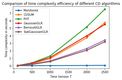
We can fit time complexity \(C^{Algorithm}(T)\) as a function of \(T\) in the form \(C(T) \simeq a T^b + c\). Using the function `scipy.optimize.curve_fit <https://docs.scipy.org/doc/scipy/reference/generated/scipy.optimize.curve_fit.html>`__, it is very easy:
[206]:
from scipy.optimize import curve_fit
[221]:
def time_complexity_general_shape(T, a, b, c):
    return a * T**b + c
[223]:
for i, alg in enumerate(all_CD_algorithms):
    popt, _ = curve_fit(time_complexity_general_shape, data_X, data_Y[i])
    a, b, c = popt
    print(f"For algorithm {alg.__name__},\n\ta = {a:.3g}, b = {b:.3g}, c = {c:.3g} is the best fit for C(T) = a T^b + c")
For algorithm Monitored,
        a = 1.96e-06, b = 1.28, c = 0.00103 is the best fit for C(T) = a T^b + c
For algorithm CUSUM,
        a = 1.21e-06, b = 1.96, c = 0.00036 is the best fit for C(T) = a T^b + c
For algorithm PHT,
        a = 5.1e-06, b = 1.82, c = -0.0397 is the best fit for C(T) = a T^b + c
For algorithm GaussianGLR,
        a = 1.44e-05, b = 1.65, c = -0.053 is the best fit for C(T) = a T^b + c
For algorithm BernoulliGLR,
        a = 2.04e-06, b = 1.83, c = 0.00612 is the best fit for C(T) = a T^b + c
For algorithm SubGaussianGLR,
        a = 7.92e-07, b = 1.94, c = 0.0144 is the best fit for C(T) = a T^b + c
We check indeed that (roughly) \(C(T^{1.3}) = \mathcal{O}(T)\) for Monitored, and \(C(T) = \mathcal{O}(T^2)\) for all the other algorithms!
Checking detection delay
[224]:
def detection_delay(data, tau, CDAlgorithm, *args, **kwargs):
    horizon = len(data)
    if isinstance(tau, float): tau = int(tau * horizon)
    for t in range(tau, horizon + 1):
        if eval_CDAlgorithm(CDAlgorithm, data, t, *args, **kwargs):
            return t - tau
    return horizon - tau
Now we can check the detection delay for our different algorithms.
For examples:
[65]:
_ = check_onemeasure(detection_delay, "Mean detection delay", firstMean=0.1, secondMean=0.4, tau=0.5, horizon=100)
Generating toy Bernoulli data for mu^1 = 0.1, mu^2 = 0.4, tau = 50 and horizon = 100...
| Algorithm | Mean detection delay |
|------|------|
| Monitored($w=80$, $b=\sqrt{\frac{w}{2} \log(2 T^2)}$) | $49.4$ |
| CUSUM($\varepsilon=0.5$, $M=50$, $h=$'auto') | $50$ |
| PHT($\varepsilon=0.5$, $M=50$, $h=$'auto') | $50$ |
| Gaussian-GLR($h_0=1$, $\delta=auto$) | $50$ |
| Bernoulli-GLR($h_0=1$, $\delta=auto$) | $50$ |
| SubGaussian-GLR($\delta=$0.01, $\sigma=$0.25, joint) | $14.1$ |
Algorithm |
Mean detection delay |
|---|---|
Monitored(\(w=80\), \(b=\sqrt{\frac{w}{2} \log(2 T^2)}\)) |
\(49.4\) |
CUSUM(\(\varepsilon=0.5\), \(M=50\), \(h=\)’auto’) |
\(50\) |
PHT(\(\varepsilon=0.5\), \(M=50\), \(h=\)’auto’) |
\(50\) |
Gaussian-GLR(\(h_0=1\), \(\delta=auto\)) |
\(50\) |
Bernoulli-GLR(\(h_0=1\), \(\delta=auto\)) |
\(50\) |
SubGaussian-GLR($:nbsphinx-math:delta`=$0.01, $:nbsphinx-math:sigma`=$0.25, joint) |
\(14.1\) |
A lot of detection delay are large (ie. it was detected too late), with not enough data! SubGaussian-GLR seems to be the only one “fast enough”, but it triggers false alarms and not correct detections!
[66]:
%%time
_ = check_onemeasure(detection_delay, "Mean detection delay", firstMean=0.1, secondMean=0.9, tau=0.5, horizon=1000)
Generating toy Bernoulli data for mu^1 = 0.1, mu^2 = 0.9, tau = 500 and horizon = 1000...
| Algorithm | Mean detection delay |
|------|------|
| Monitored($w=80$, $b=\sqrt{\frac{w}{2} \log(2 T^2)}$) | $31.7$ |
| CUSUM($\varepsilon=0.5$, $M=50$, $h=$'auto') | $37.9$ |
| PHT($\varepsilon=0.5$, $M=50$, $h=$'auto') | $41.8$ |
| Gaussian-GLR($h_0=1$, $\delta=auto$) | $30.3$ |
| Bernoulli-GLR($h_0=1$, $\delta=auto$) | $22.7$ |
| SubGaussian-GLR($\delta=$0.01, $\sigma=$0.25, joint) | $3.86$ |
Algorithm |
Mean detection delay |
|---|---|
Monitored(\(w=80\), \(b=\sqrt{\frac{w}{2} \log(2 T^2)}\)) |
\(31.7\) |
CUSUM(\(\varepsilon=0.5\), \(M=50\), \(h=\)’auto’) |
\(37.9\) |
PHT(\(\varepsilon=0.5\), \(M=50\), \(h=\)’auto’) |
\(41.8\) |
Gaussian-GLR(\(h_0=1\), \(\delta=auto\)) |
\(30.3\) |
Bernoulli-GLR(\(h_0=1\), \(\delta=auto\)) |
\(22.7\) |
SubGaussian-GLR($:nbsphinx-math:delta`=$0.01, $:nbsphinx-math:sigma`=$0.25, joint) |
\(3.86\) |
CPU times: user 20.1 s, sys: 149 ms, total: 20.2 s
Wall time: 20.1 s
A very small detection delay, with enough data (a delay of 40 is small when there is \(500\) data of \(\nu_1\) and \(\nu_2\)) !
Checking false alarm probabilities
[225]:
def false_alarm(data, tau, CDAlgorithm, *args, **kwargs):
    horizon = len(data)
    if isinstance(tau, float): tau = int(tau * horizon)
    for t in range(0, tau):
        if eval_CDAlgorithm(CDAlgorithm, data, t, *args, **kwargs):
            return True
    return False
Now we can check the false alarm probabilities for our different algorithms.
For examples:
[68]:
_ = check_onemeasure(false_alarm, "Mean false alarm rate", firstMean=0.1, secondMean=0.4, tau=0.5, horizon=100)
Generating toy Bernoulli data for mu^1 = 0.1, mu^2 = 0.4, tau = 50 and horizon = 100...
| Algorithm | Mean false alarm rate |
|------|------|
| Monitored($w=80$, $b=\sqrt{\frac{w}{2} \log(2 T^2)}$) | $0$ |
| CUSUM($\varepsilon=0.5$, $M=50$, $h=$'auto') | $0$ |
| PHT($\varepsilon=0.5$, $M=50$, $h=$'auto') | $0$ |
| Gaussian-GLR($h_0=1$, $\delta=auto$) | $0$ |
| Bernoulli-GLR($h_0=1$, $\delta=auto$) | $0$ |
| SubGaussian-GLR($\delta=$0.01, $\sigma=$0.25, joint) | $0.1$ |
Algorithm |
Mean false alarm rate |
|---|---|
Monitored(\(w=80\), \(b=\sqrt{\frac{w}{2} \log(2 T^2)}\)) |
\(0\) |
CUSUM(\(\varepsilon=0.5\), \(M=50\), \(h=\)’auto’) |
\(0\) |
PHT(\(\varepsilon=0.5\), \(M=50\), \(h=\)’auto’) |
\(0\) |
Gaussian-GLR(\(h_0=1\), \(\delta=auto\)) |
\(0\) |
Bernoulli-GLR(\(h_0=1\), \(\delta=auto\)) |
\(0\) |
SubGaussian-GLR($:nbsphinx-math:delta`=$0.01, $:nbsphinx-math:sigma`=$0.25, joint) |
\(0.1\) |
A lot of false alarm for BernoulliGLR but not the others, with not enough data!
[69]:
%%time
_ = check_onemeasure(false_alarm, "Mean false alarm rate", firstMean=0.1, secondMean=0.9, tau=0.5, horizon=1000)
Generating toy Bernoulli data for mu^1 = 0.1, mu^2 = 0.9, tau = 500 and horizon = 1000...
| Algorithm | Mean false alarm rate |
|------|------|
| Monitored($w=80$, $b=\sqrt{\frac{w}{2} \log(2 T^2)}$) | $0$ |
| CUSUM($\varepsilon=0.5$, $M=50$, $h=$'auto') | $0$ |
| PHT($\varepsilon=0.5$, $M=50$, $h=$'auto') | $0$ |
| Gaussian-GLR($h_0=1$, $\delta=auto$) | $0$ |
| Bernoulli-GLR($h_0=1$, $\delta=auto$) | $0$ |
| SubGaussian-GLR($\delta=$0.01, $\sigma=$0.25, joint) | $0.48$ |
Algorithm |
Mean false alarm rate |
|---|---|
Monitored(\(w=80\), \(b=\sqrt{\frac{w}{2} \log(2 T^2)}\)) |
\(0\) |
CUSUM(\(\varepsilon=0.5\), \(M=50\), \(h=\)’auto’) |
\(0\) |
PHT(\(\varepsilon=0.5\), \(M=50\), \(h=\)’auto’) |
\(0\) |
Gaussian-GLR(\(h_0=1\), \(\delta=auto\)) |
\(0\) |
Bernoulli-GLR(\(h_0=1\), \(\delta=auto\)) |
\(0\) |
SubGaussian-GLR($:nbsphinx-math:delta`=$0.01, $:nbsphinx-math:sigma`=$0.25, joint) |
\(0.48\) |
CPU times: user 3min 1s, sys: 198 ms, total: 3min 1s
Wall time: 3min 1s
No false alarm, with enough data! Only Sub-Gaussian-GLR has a lot of false alarms, even with enough data!
Checking missed detection probabilities
[226]:
def missed_detection(data, tau, CDAlgorithm, *args, **kwargs):
    horizon = len(data)
    if isinstance(tau, float): tau = int(tau * horizon)
    for t in range(tau, horizon + 1):
        if eval_CDAlgorithm(CDAlgorithm, data, t, *args, **kwargs):
            return False
    return True
Now we can check the false alarm probabilities for our different algorithms.
For examples:
[71]:
_ = check_onemeasure(missed_detection, "Mean missed detection rate", firstMean=0.1, secondMean=0.4, tau=0.5, horizon=100)
Generating toy Bernoulli data for mu^1 = 0.1, mu^2 = 0.4, tau = 50 and horizon = 100...
| Algorithm | Mean missed detection rate |
|------|------|
| Monitored($w=80$, $b=\sqrt{\frac{w}{2} \log(2 T^2)}$) | $0.96$ |
| CUSUM($\varepsilon=0.5$, $M=50$, $h=$'auto') | $1$ |
| PHT($\varepsilon=0.5$, $M=50$, $h=$'auto') | $1$ |
| Gaussian-GLR($h_0=1$, $\delta=auto$) | $1$ |
| Bernoulli-GLR($h_0=1$, $\delta=auto$) | $1$ |
| SubGaussian-GLR($\delta=$0.01, $\sigma=$0.25, joint) | $0$ |
Algorithm |
Mean missed detection rate |
|---|---|
Monitored(\(w=80\), \(b=\sqrt{\frac{w}{2} \log(2 T^2)}\)) |
\(0.96\) |
CUSUM(\(\varepsilon=0.5\), \(M=50\), \(h=\)’auto’) |
\(1\) |
PHT(\(\varepsilon=0.5\), \(M=50\), \(h=\)’auto’) |
\(1\) |
Gaussian-GLR(\(h_0=1\), \(\delta=auto\)) |
\(1\) |
Bernoulli-GLR(\(h_0=1\), \(\delta=auto\)) |
\(1\) |
SubGaussian-GLR($:nbsphinx-math:delta`=$0.01, $:nbsphinx-math:sigma`=$0.25, joint) |
\(0\) |
A lot of missed detection, with not enough data!
[72]:
%%time
_ = check_onemeasure(missed_detection, "Mean missed detection rate", firstMean=0.1, secondMean=0.9, tau=0.5, horizon=1000)
Generating toy Bernoulli data for mu^1 = 0.1, mu^2 = 0.9, tau = 500 and horizon = 1000...
| Algorithm | Mean missed detection rate |
|------|------|
| Monitored($w=80$, $b=\sqrt{\frac{w}{2} \log(2 T^2)}$) | $0$ |
| CUSUM($\varepsilon=0.5$, $M=50$, $h=$'auto') | $0$ |
| PHT($\varepsilon=0.5$, $M=50$, $h=$'auto') | $0$ |
| Gaussian-GLR($h_0=1$, $\delta=auto$) | $0$ |
| Bernoulli-GLR($h_0=1$, $\delta=auto$) | $0$ |
| SubGaussian-GLR($\delta=$0.01, $\sigma=$0.25, joint) | $0$ |
Algorithm |
Mean missed detection rate |
|---|---|
Monitored(\(w=80\), \(b=\sqrt{\frac{w}{2} \log(2 T^2)}\)) |
\(0\) |
CUSUM(\(\varepsilon=0.5\), \(M=50\), \(h=\)’auto’) |
\(0\) |
PHT(\(\varepsilon=0.5\), \(M=50\), \(h=\)’auto’) |
\(0\) |
Gaussian-GLR(\(h_0=1\), \(\delta=auto\)) |
\(0\) |
Bernoulli-GLR(\(h_0=1\), \(\delta=auto\)) |
\(0\) |
SubGaussian-GLR($:nbsphinx-math:delta`=$0.01, $:nbsphinx-math:sigma`=$0.25, joint) |
\(0\) |
CPU times: user 20.7 s, sys: 200 ms, total: 20.9 s
Wall time: 20.7 s
No missed detection, with enough data!
More simulations and some plots
Run a check for a grid of values
Fix an algorithm, e.g., Monitored, then consider one of the quantities defined above (time efficiency, delay, false alarm or missed detection probas). Now, a piecewise stationary problem is characterized by the parameters \(\mu_1\), \(\Delta = |\mu_2 - \mu_1|\), and \(\tau\) and \(T\).
Fix \(\mu_1=\frac12\), and so \(\Delta\) can be taken anywhere in \([0, \frac12]\).
Fix \(T=1000\) for instance, and so \(\tau\) can be taken anywhere in \([0,T]\).
Of course, if any of \(\tau\) or \(\Delta\) are too small, detection is impossible. I want to display a \(2\)D image view, showing on \(x\)-axis a grid of values of \(\Delta\), on \(y\)-axis a grid of values of \(\tau\), and on the \(2\)D image, a color-scale to show the detection delay (for instance).
[230]:
mu_1 = 0.5
max_mu_2 = 1
nb_values_Delta = 20
values_Delta = np.linspace(0, max_mu_2 - mu_1, nb_values_Delta)
[231]:
horizon = T = 1000
min_tau = 10
max_tau = T - min_tau
step = 50
values_tau = np.arange(min_tau, max_tau + 1, step)
nb_values_tau = len(values_tau)
[232]:
print(f"This will give a grid of {nb_values_Delta} x {nb_values_tau} = {nb_values_Delta * nb_values_tau} values of Delta and tau to explore.")
This will give a grid of 20 x 20 = 400 values of Delta and tau to explore.
And now the function:
[233]:
def check2D_onemeasure(measure,
                       CDAlgorithm,
                       values_Delta,
                       values_tau,
                       firstMean=mu_1,
                       horizon=horizon,
                       repetitions=10,
                       verbose=True,
                       gaussian=False,
                       n_jobs=1,
                       *args, **kwargs,
    ):
    print(f"\nExploring {measure.__name__} for algorithm {str_of_CDAlgorithm(CDAlgorithm, *args, **kwargs)} mu^1 = {firstMean} and horizon = {horizon}...")
    nb_values_Delta = len(values_Delta)
    nb_values_tau = len(values_tau)
    print(f"with {nb_values_Delta} values for Delta, and {nb_values_tau} values for tau, and {repetitions} repetitions.")
    results = np.zeros((nb_values_Delta, nb_values_tau))

    for i, delta in tqdm(enumerate(values_Delta), desc="Delta s", leave=False):
        for j, tau in tqdm(enumerate(values_tau), desc="Tau s", leave=False):
            secondMean = firstMean + delta
            if isinstance(tau, float): tau = int(tau * horizon)

            # now the random Monte Carlo repetitions
            for rep in tqdm(range(repetitions), desc="Repetitions", leave=False):
                data = get_toy_data(firstMean=firstMean, secondMean=secondMean, tau=tau, horizon=horizon, gaussian=gaussian)
                result = measure(data, tau, CDAlgorithm, *args, **kwargs)
                results[i, j] += result
            results[i, j] /= repetitions
            if verbose: print(f"For delta = {delta} ({i}th), tau = {tau} ({j}th), mean result = {results[i, j]}")
    return results
A version using joblib.Parallel to use multi-core computations
I want to (try to) use `joblib.Parallel <https://joblib.readthedocs.io/en/latest/parallel.html>`__ to run the “repetitions” for loop in parallel, for instance on 4 cores on my machine.
[234]:
from joblib import Parallel, delayed
[235]:
# Tries to know number of CPU
try:
    from multiprocessing import cpu_count
    CPU_COUNT = cpu_count()  #: Number of CPU on the local machine
except ImportError:
    CPU_COUNT = 1
print(f"Info: using {CPU_COUNT} jobs in parallel!")
Info: using 4 jobs in parallel!
We can rewrite the check2D_onemeasure function to run some loops in parallel.
[236]:
def check2D_onemeasure_parallel(measure,
                                CDAlgorithm,
                                values_Delta,
                                values_tau,
                                firstMean=mu_1,
                                horizon=horizon,
                                repetitions=10,
                                verbose=1,
                                gaussian=False,
                                n_jobs=CPU_COUNT,
                                *args, **kwargs,
    ):
    print(f"\nExploring {measure.__name__} for algorithm {str_of_CDAlgorithm(CDAlgorithm, *args, **kwargs)} mu^1 = {firstMean} and horizon = {horizon}...")
    nb_values_Delta = len(values_Delta)
    nb_values_tau = len(values_tau)
    print(f"with {nb_values_Delta} values for Delta, and {nb_values_tau} values for tau, and {repetitions} repetitions.")
    results = np.zeros((nb_values_Delta, nb_values_tau))

    def delayed_measure(i, delta, j, tau, rep):
        secondMean = firstMean + delta
        if isinstance(tau, float): tau = int(tau * horizon)
        data = get_toy_data(firstMean=firstMean, secondMean=secondMean, tau=tau, horizon=horizon, gaussian=gaussian)
        return i, j, measure(data, tau, CDAlgorithm, *args, **kwargs)

    # now the random Monte Carlo repetitions
    for i, j, result in Parallel(n_jobs=n_jobs, verbose=int(verbose))(
        delayed(delayed_measure)(i, delta, j, tau, rep)
        for i, delta in tqdm(enumerate(values_Delta), desc="Delta s ||",    leave=False)
        for j, tau   in tqdm(enumerate(values_tau),   desc="Tau s ||",      leave=False)
        for rep      in tqdm(range(repetitions),      desc="Repetitions||", leave=False)
    ):
        results[i, j] += result
    results /= repetitions

    if verbose:
        for i, delta in enumerate(values_Delta):
            for j, tau in enumerate(values_tau):
                print(f"For delta = {delta} ({i}th), tau = {tau} ({j}th), mean result = {results[i, j]}")
    return results
Checking on a small grid of values
[80]:
Monitored
[80]:
__main__.Monitored
[233]:
%%time
_ = check2D_onemeasure(time_efficiency,
                       Monitored,
                       values_Delta=[0.05, 0.25, 0.5],
                       values_tau=[1/10, 1/4, 2/4, 3/4, 9/10],
                       firstMean=0.5,
                       horizon=1000,
                       repetitions=100)
Exploring time_efficiency for algorithm Monitored($w=80$, $b=\sqrt{\frac{w}{2} \log(2 T^2)}$) mu^1 = 0.5 and horizon = 1000...
with 3 values for Delta, and 5 values for tau, and 100 repetitions.
For delta = 0.05 (0th), tau = 100 (0th), mean result = 0.018056981563568116
For delta = 0.05 (0th), tau = 250 (1th), mean result = 0.017168304920196532
For delta = 0.05 (0th), tau = 500 (2th), mean result = 0.01913909912109375
For delta = 0.05 (0th), tau = 750 (3th), mean result = 0.027340266704559326
For delta = 0.05 (0th), tau = 900 (4th), mean result = 0.023344976902008055
For delta = 0.25 (1th), tau = 100 (0th), mean result = 0.023643691539764405
For delta = 0.25 (1th), tau = 250 (1th), mean result = 0.03245354175567627
For delta = 0.25 (1th), tau = 500 (2th), mean result = 0.032449700832366944
For delta = 0.25 (1th), tau = 750 (3th), mean result = 0.018729052543640136
For delta = 0.25 (1th), tau = 900 (4th), mean result = 0.026870133876800536
For delta = 0.5 (2th), tau = 100 (0th), mean result = 0.02412700653076172
For delta = 0.5 (2th), tau = 250 (1th), mean result = 0.025472092628479003
For delta = 0.5 (2th), tau = 500 (2th), mean result = 0.019556210041046143
For delta = 0.5 (2th), tau = 750 (3th), mean result = 0.01786205768585205
For delta = 0.5 (2th), tau = 900 (4th), mean result = 0.019401206970214843
CPU times: user 45.5 s, sys: 1.88 s, total: 47.4 s
Wall time: 46.6 s
[82]:
%%time
_ = check2D_onemeasure_parallel(time_efficiency,
                                Monitored,
                                values_Delta=[0.05, 0.25, 0.5],
                                values_tau=[1/10, 1/4, 2/4, 3/4, 9/10],
                                firstMean=0.5,
                                horizon=1000,
                                repetitions=100,
                                n_jobs=4)
Exploring time_efficiency for algorithm Monitored($w=80$, $b=\sqrt{\frac{w}{2} \log(2 T^2)}$) mu^1 = 0.5 and horizon = 1000...
with 3 values for Delta, and 5 values for tau, and 100 repetitions.
[Parallel(n_jobs=4)]: Using backend LokyBackend with 4 concurrent workers.
[Parallel(n_jobs=4)]: Done 110 tasks | elapsed: 1.9s
[Parallel(n_jobs=4)]: Done 1010 tasks | elapsed: 11.4s
For delta = 0.05 (0th), tau = 0.1 (0th), mean result = 0.034742271900177
For delta = 0.05 (0th), tau = 0.25 (1th), mean result = 0.03206165313720703
For delta = 0.05 (0th), tau = 0.5 (2th), mean result = 0.03520160436630249
For delta = 0.05 (0th), tau = 0.75 (3th), mean result = 0.03601207733154297
For delta = 0.05 (0th), tau = 0.9 (4th), mean result = 0.036164679527282716
For delta = 0.25 (1th), tau = 0.1 (0th), mean result = 0.03190211772918701
For delta = 0.25 (1th), tau = 0.25 (1th), mean result = 0.03288561344146729
For delta = 0.25 (1th), tau = 0.5 (2th), mean result = 0.032886896133422855
For delta = 0.25 (1th), tau = 0.75 (3th), mean result = 0.03128063201904297
For delta = 0.25 (1th), tau = 0.9 (4th), mean result = 0.03194632768630981
For delta = 0.5 (2th), tau = 0.1 (0th), mean result = 0.03349523544311524
For delta = 0.5 (2th), tau = 0.25 (1th), mean result = 0.03411170482635498
For delta = 0.5 (2th), tau = 0.5 (2th), mean result = 0.03451453685760498
For delta = 0.5 (2th), tau = 0.75 (3th), mean result = 0.03463083505630493
For delta = 0.5 (2th), tau = 0.9 (4th), mean result = 0.03331227302551269
CPU times: user 1.05 s, sys: 121 ms, total: 1.17 s
Wall time: 16.5 s
[Parallel(n_jobs=4)]: Done 1500 out of 1500 | elapsed: 16.4s finished
[83]:
%%time
_ = check2D_onemeasure(detection_delay,
                       Monitored,
                       values_Delta=[0.05, 0.25, 0.5],
                       values_tau=[1/10, 1/4, 2/4, 3/4, 9/10],
                       firstMean=0.5,
                       horizon=1000,
                       repetitions=100)
Exploring detection_delay for algorithm Monitored($w=80$, $b=\sqrt{\frac{w}{2} \log(2 T^2)}$) mu^1 = 0.5 and horizon = 1000...
with 3 values for Delta, and 5 values for tau, and 100 repetitions.
For delta = 0.05 (0th), tau = 100 (0th), mean result = 900.0
For delta = 0.05 (0th), tau = 250 (1th), mean result = 750.0
For delta = 0.05 (0th), tau = 500 (2th), mean result = 500.0
For delta = 0.05 (0th), tau = 750 (3th), mean result = 250.0
For delta = 0.05 (0th), tau = 900 (4th), mean result = 100.0
For delta = 0.25 (1th), tau = 100 (0th), mean result = 900.0
For delta = 0.25 (1th), tau = 250 (1th), mean result = 750.0
For delta = 0.25 (1th), tau = 500 (2th), mean result = 500.0
For delta = 0.25 (1th), tau = 750 (3th), mean result = 250.0
For delta = 0.25 (1th), tau = 900 (4th), mean result = 100.0
For delta = 0.5 (2th), tau = 100 (0th), mean result = 753.63
For delta = 0.5 (2th), tau = 250 (1th), mean result = 671.52
For delta = 0.5 (2th), tau = 500 (2th), mean result = 458.34
For delta = 0.5 (2th), tau = 750 (3th), mean result = 228.66
For delta = 0.5 (2th), tau = 900 (4th), mean result = 93.58
CPU times: user 19.3 s, sys: 1.25 s, total: 20.5 s
Wall time: 18.9 s
[84]:
%%time
_ = check2D_onemeasure_parallel(detection_delay,
                                Monitored,
                                values_Delta=[0.05, 0.25, 0.5],
                                values_tau=[1/10, 1/4, 2/4, 3/4, 9/10],
                                firstMean=0.5,
                                horizon=1000,
                                repetitions=100
                               )
Exploring detection_delay for algorithm Monitored($w=80$, $b=\sqrt{\frac{w}{2} \log(2 T^2)}$) mu^1 = 0.5 and horizon = 1000...
with 3 values for Delta, and 5 values for tau, and 100 repetitions.
[Parallel(n_jobs=4)]: Using backend LokyBackend with 4 concurrent workers.
[Parallel(n_jobs=4)]: Done 280 tasks | elapsed: 3.0s
For delta = 0.05 (0th), tau = 0.1 (0th), mean result = 900.0
For delta = 0.05 (0th), tau = 0.25 (1th), mean result = 750.0
For delta = 0.05 (0th), tau = 0.5 (2th), mean result = 500.0
For delta = 0.05 (0th), tau = 0.75 (3th), mean result = 250.0
For delta = 0.05 (0th), tau = 0.9 (4th), mean result = 100.0
For delta = 0.25 (1th), tau = 0.1 (0th), mean result = 900.0
For delta = 0.25 (1th), tau = 0.25 (1th), mean result = 750.0
For delta = 0.25 (1th), tau = 0.5 (2th), mean result = 500.0
For delta = 0.25 (1th), tau = 0.75 (3th), mean result = 250.0
For delta = 0.25 (1th), tau = 0.9 (4th), mean result = 100.0
For delta = 0.5 (2th), tau = 0.1 (0th), mean result = 813.76
For delta = 0.5 (2th), tau = 0.25 (1th), mean result = 657.41
For delta = 0.5 (2th), tau = 0.5 (2th), mean result = 439.97
For delta = 0.5 (2th), tau = 0.75 (3th), mean result = 233.06
For delta = 0.5 (2th), tau = 0.9 (4th), mean result = 94.97
CPU times: user 975 ms, sys: 42.1 ms, total: 1.02 s
Wall time: 19.2 s
[Parallel(n_jobs=4)]: Done 1500 out of 1500 | elapsed: 19.2s finished
[85]:
%%time
_ = check2D_onemeasure_parallel(false_alarm,
                                Monitored,
                                values_Delta=[0.05, 0.25, 0.5],
                                values_tau=[1/10, 1/4, 2/4, 3/4, 9/10],
                                firstMean=0.5,
                                horizon=1000,
                                repetitions=100,
                                )
Exploring false_alarm for algorithm Monitored($w=80$, $b=\sqrt{\frac{w}{2} \log(2 T^2)}$) mu^1 = 0.5 and horizon = 1000...
with 3 values for Delta, and 5 values for tau, and 100 repetitions.
[Parallel(n_jobs=4)]: Using backend LokyBackend with 4 concurrent workers.
[Parallel(n_jobs=4)]: Done 852 tasks | elapsed: 6.3s
For delta = 0.05 (0th), tau = 0.1 (0th), mean result = 0.0
For delta = 0.05 (0th), tau = 0.25 (1th), mean result = 0.0
For delta = 0.05 (0th), tau = 0.5 (2th), mean result = 0.0
For delta = 0.05 (0th), tau = 0.75 (3th), mean result = 0.0
For delta = 0.05 (0th), tau = 0.9 (4th), mean result = 0.0
For delta = 0.25 (1th), tau = 0.1 (0th), mean result = 0.0
For delta = 0.25 (1th), tau = 0.25 (1th), mean result = 0.0
For delta = 0.25 (1th), tau = 0.5 (2th), mean result = 0.0
For delta = 0.25 (1th), tau = 0.75 (3th), mean result = 0.0
For delta = 0.25 (1th), tau = 0.9 (4th), mean result = 0.0
For delta = 0.5 (2th), tau = 0.1 (0th), mean result = 0.0
For delta = 0.5 (2th), tau = 0.25 (1th), mean result = 0.0
For delta = 0.5 (2th), tau = 0.5 (2th), mean result = 0.0
For delta = 0.5 (2th), tau = 0.75 (3th), mean result = 0.0
For delta = 0.5 (2th), tau = 0.9 (4th), mean result = 0.0
CPU times: user 820 ms, sys: 41.8 ms, total: 861 ms
Wall time: 11.5 s
[Parallel(n_jobs=4)]: Done 1500 out of 1500 | elapsed: 11.4s finished
[86]:
%%time
_ = check2D_onemeasure_parallel(missed_detection,
                                Monitored,
                                values_Delta=[0.05, 0.25, 0.5],
                                values_tau=[1/10, 1/4, 2/4, 3/4, 9/10],
                                firstMean=0.5,
                                horizon=1000,
                                repetitions=100,
                                )
Exploring missed_detection for algorithm Monitored($w=80$, $b=\sqrt{\frac{w}{2} \log(2 T^2)}$) mu^1 = 0.5 and horizon = 1000...
with 3 values for Delta, and 5 values for tau, and 100 repetitions.
[Parallel(n_jobs=4)]: Using backend LokyBackend with 4 concurrent workers.
[Parallel(n_jobs=4)]: Done 348 tasks | elapsed: 3.5s
For delta = 0.05 (0th), tau = 0.1 (0th), mean result = 1.0
For delta = 0.05 (0th), tau = 0.25 (1th), mean result = 1.0
For delta = 0.05 (0th), tau = 0.5 (2th), mean result = 1.0
For delta = 0.05 (0th), tau = 0.75 (3th), mean result = 1.0
For delta = 0.05 (0th), tau = 0.9 (4th), mean result = 1.0
For delta = 0.25 (1th), tau = 0.1 (0th), mean result = 1.0
For delta = 0.25 (1th), tau = 0.25 (1th), mean result = 1.0
For delta = 0.25 (1th), tau = 0.5 (2th), mean result = 1.0
For delta = 0.25 (1th), tau = 0.75 (3th), mean result = 1.0
For delta = 0.25 (1th), tau = 0.9 (4th), mean result = 1.0
For delta = 0.5 (2th), tau = 0.1 (0th), mean result = 0.93
For delta = 0.5 (2th), tau = 0.25 (1th), mean result = 0.91
For delta = 0.5 (2th), tau = 0.5 (2th), mean result = 0.89
For delta = 0.5 (2th), tau = 0.75 (3th), mean result = 0.92
For delta = 0.5 (2th), tau = 0.9 (4th), mean result = 0.83
CPU times: user 930 ms, sys: 44.8 ms, total: 974 ms
Wall time: 11.6 s
[Parallel(n_jobs=4)]: Done 1500 out of 1500 | elapsed: 11.6s finished
Plotting the result as a 2D image
[238]:
import matplotlib as mpl
FIGSIZE = (19.80, 10.80)  #: Figure size, in inches!
mpl.rcParams['figure.figsize'] = FIGSIZE
import matplotlib.ticker as ticker
import matplotlib.pyplot as plt
[239]:
#: List of formats to use for saving the figures, by default.
#: It is a smart idea to save in both a raster and vectorial formats
FORMATS = ('png', 'pdf')

import pickle
from datetime import datetime
from os.path import getsize, getatime


def show_and_save(showplot=True, savefig=None, formats=FORMATS, pickleit=False, fig=None):
    """ Maximize the window if need to show it, save it if needed, and then show it or close it.

    - Inspired by https://tomspur.blogspot.fr/2015/08/publication-ready-figures-with.html#Save-the-figure
    """
    if savefig is not None:
        if pickleit and fig is not None:
            form = "pickle"
            path = "{}.{}".format(savefig, form)
            print("Saving raw figure with format {}, to file '{}'...".format(form, path))  # DEBUG
            with open(path, "bw") as f:
                pickle_dump(fig, f)
            print("       Saved! '{}' created of size '{}b', at '{:%c}' ...".format(path, getsize(path), datetime.fromtimestamp(getatime(path))))
        for form in formats:
            path = "{}.{}".format(savefig, form)
            print("Saving figure with format {}, to file '{}'...".format(form, path))  # DEBUG
            plt.savefig(path, bbox_inches=None)
            print("       Saved! '{}' created of size '{}b', at '{:%c}' ...".format(path, getsize(path), datetime.fromtimestamp(getatime(path))))
    try:
        plt.show() if showplot else plt.close()
    except (TypeError, AttributeError):
        print("Failed to show the figure for some unknown reason...")  # DEBUG
Now the function:
[240]:
def view2D_onemeasure(measure, name,
                      CDAlgorithm,
                      values_Delta,
                      values_tau,
                      firstMean=mu_1,
                      horizon=horizon,
                      repetitions=10,
                      gaussian=False,
                      n_jobs=CPU_COUNT,
                      savefig=None,
                      *args, **kwargs,
    ):
    check = check2D_onemeasure_parallel if n_jobs > 1 else check2D_onemeasure
    results = check(measure, CDAlgorithm,
                    values_Delta, values_tau,
                    firstMean=firstMean,
                    horizon=horizon,
                    repetitions=repetitions,
                    verbose=False,
                    gaussian=gaussian,
                    n_jobs=n_jobs,
                    *args, **kwargs,
    )
    fig = plt.figure()

    plt.matshow(results)
    plt.colorbar(shrink=0.7)

    plt.locator_params(axis='x', nbins=1+len(values_tau))
    plt.locator_params(axis='y', nbins=len(values_Delta))

    ax = plt.gca()
    # https://stackoverflow.com/a/19972993/
    loc = ticker.MultipleLocator(base=1.0) # this locator puts ticks at regular intervals
    ax.xaxis.set_major_locator(loc)
    ax.xaxis.set_ticks_position('bottom')
    def y_fmt(tick_value, pos): return '{:.3g}'.format(tick_value)
    ax.yaxis.set_major_formatter(ticker.FuncFormatter(y_fmt))
    ax.yaxis.set_major_locator(loc)

    # hack to display the ticks labels as the actual values
    if np.max(values_tau) <= 1:
        values_tau = np.floor(np.asarray(values_tau) * horizon)
        values_tau = list(np.asarray(values_tau, dtype=int))
    values_Delta = np.round(values_Delta, 3)
    ax.set_xticklabels([0] + list(values_tau))  # hack: the first label is not displayed??
    ax.set_yticklabels([0] + list(values_Delta))  # hack: the first label is not displayed??

    plt.title(fr"{name} for algorithm {str_of_CDAlgorithm(CDAlgorithm, *args, **kwargs)}, for $T={horizon}$, {'Gaussian' if gaussian else 'Bernoulli'} data and $\mu_1={firstMean:.3g}$ and ${repetitions}$ repetitions")
    plt.xlabel(r"Value of $\tau$ time of breakpoint")
    plt.ylabel(r"Value of gap $\Delta = |\mu_2 - \mu_1|$")


    show_and_save(savefig=savefig)
    return fig
First example
For Monitored
[110]:
%%time
_ = view2D_onemeasure(detection_delay, "Detection delay",
                      Monitored,
                      values_Delta=[0.05, 0.1, 0.25, 0.4, 0.5],
                      values_tau=[1/10, 1/4, 2/4, 3/4, 9/10],
                      firstMean=0.5,
                      horizon=1000,
                      repetitions=50,
                      savefig="Detection_delay_of_Monitored__Bernoulli_T1000_N50__5deltas__5taus"
                     )
Exploring detection_delay for algorithm Monitored($w=80$, $b=\sqrt{\frac{w}{2} \log(2 T^2)}$) mu^1 = 0.5 and horizon = 1000...
with 5 values for Delta, and 5 values for tau, and 50 repetitions.
Saving figure with format png, to file 'Detection_delay_of_Monitored__Bernoulli_T1000_N50__5deltas__5taus.png'...
       Saved! 'Detection_delay_of_Monitored__Bernoulli_T1000_N50__5deltas__5taus.png' created of size '24517b', at 'Sun Dec 16 22:41:23 2018' ...
Saving figure with format pdf, to file 'Detection_delay_of_Monitored__Bernoulli_T1000_N50__5deltas__5taus.pdf'...
       Saved! 'Detection_delay_of_Monitored__Bernoulli_T1000_N50__5deltas__5taus.pdf' created of size '25149b', at 'Sun Dec 16 22:42:43 2018' ...
<Figure size 1425.6x777.6 with 0 Axes>
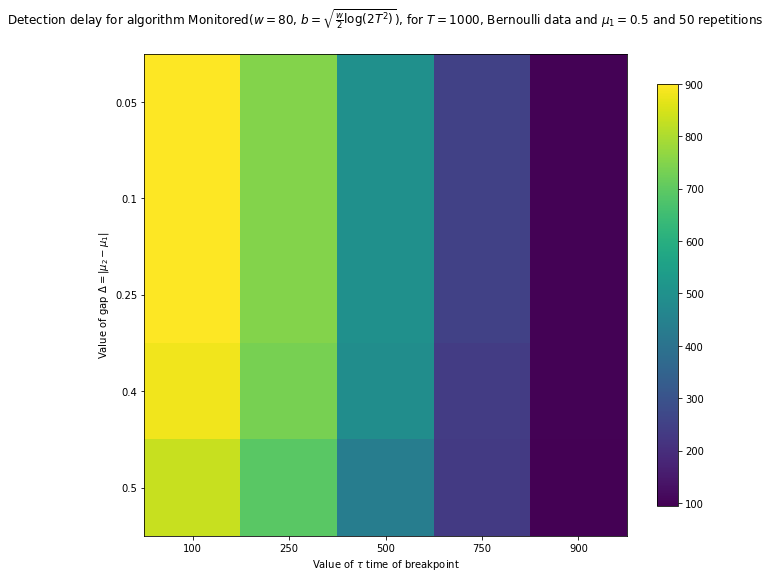
CPU times: user 2.61 s, sys: 833 ms, total: 3.45 s
Wall time: 10.3 s
[118]:
%%time
_ = view2D_onemeasure(false_alarm, "False alarm probability",
                      Monitored,
                      values_Delta=[0.05, 0.1, 0.25, 0.4, 0.5],
                      values_tau=[1/10, 1/4, 2/4, 3/4, 9/10],
                      firstMean=0.5,
                      horizon=1000,
                      repetitions=50,
                      savefig="False_alarm_of_Monitored__Bernoulli_T1000_N50__5deltas__5taus"
                     )
Exploring false_alarm for algorithm Monitored($w=80$, $b=\sqrt{\frac{w}{2} \log(2 T^2)}$) mu^1 = 0.5 and horizon = 1000...
with 5 values for Delta, and 5 values for tau, and 50 repetitions.
Saving figure with format png, to file 'False_alarm_of_Monitored__Bernoulli_T1000_N50__5deltas__5taus.png'...
       Saved! 'False_alarm_of_Monitored__Bernoulli_T1000_N50__5deltas__5taus.png' created of size '25190b', at 'Sun Dec 16 22:46:49 2018' ...
Saving figure with format pdf, to file 'False_alarm_of_Monitored__Bernoulli_T1000_N50__5deltas__5taus.pdf'...
       Saved! 'False_alarm_of_Monitored__Bernoulli_T1000_N50__5deltas__5taus.pdf' created of size '23765b', at 'Sun Dec 16 22:46:49 2018' ...
<Figure size 1425.6x777.6 with 0 Axes>
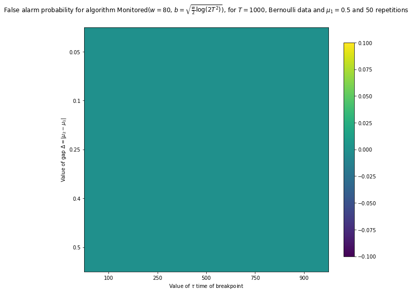
CPU times: user 2.63 s, sys: 1.23 s, total: 3.86 s
Wall time: 9.77 s
[119]:
%%time
_ = view2D_onemeasure(missed_detection, "Missed detection probability",
                      Monitored,
                      values_Delta=[0.05, 0.1, 0.25, 0.4, 0.5],
                      values_tau=[1/10, 1/4, 2/4, 3/4, 9/10],
                      firstMean=0.5,
                      horizon=1000,
                      repetitions=50,
                      savefig="Missed_detection_of_Monitored__Bernoulli_T1000_N50__5deltas__5taus"
                     )
Exploring missed_detection for algorithm Monitored($w=80$, $b=\sqrt{\frac{w}{2} \log(2 T^2)}$) mu^1 = 0.5 and horizon = 1000...
with 5 values for Delta, and 5 values for tau, and 50 repetitions.
Saving figure with format png, to file 'Missed_detection_of_Monitored__Bernoulli_T1000_N50__5deltas__5taus.png'...
       Saved! 'Missed_detection_of_Monitored__Bernoulli_T1000_N50__5deltas__5taus.png' created of size '24349b', at 'Sun Dec 16 22:47:50 2018' ...
Saving figure with format pdf, to file 'Missed_detection_of_Monitored__Bernoulli_T1000_N50__5deltas__5taus.pdf'...
       Saved! 'Missed_detection_of_Monitored__Bernoulli_T1000_N50__5deltas__5taus.pdf' created of size '24377b', at 'Sun Dec 16 22:47:50 2018' ...
<Figure size 1425.6x777.6 with 0 Axes>
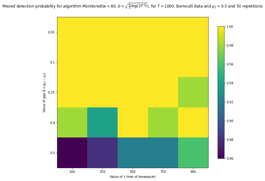
CPU times: user 2.6 s, sys: 1.14 s, total: 3.74 s
Wall time: 10.1 s
[121]:
%%time
_ = view2D_onemeasure(false_alarm, "False alarm probability",
                      Monitored,
                      values_Delta=[0.05, 0.1, 0.25, 0.4, 0.5],
                      values_tau=[1/10, 1/4, 2/4, 3/4, 9/10],
                      firstMean=0.5,
                      horizon=1000,
                      repetitions=50,
                      gaussian=True,
                      savefig="False_alarm_of_Monitored__Gaussian_T1000_N50__5deltas__5taus"
                     )
Exploring false_alarm for algorithm Monitored($w=80$, $b=\sqrt{\frac{w}{2} \log(2 T^2)}$) mu^1 = 0.5 and horizon = 1000...
with 5 values for Delta, and 5 values for tau, and 50 repetitions.
Saving figure with format png, to file 'False_alarm_of_Monitored__Gaussian_T1000_N50__5deltas__5taus.png'...
       Saved! 'False_alarm_of_Monitored__Gaussian_T1000_N50__5deltas__5taus.png' created of size '25249b', at 'Sun Dec 16 22:50:50 2018' ...
Saving figure with format pdf, to file 'False_alarm_of_Monitored__Gaussian_T1000_N50__5deltas__5taus.pdf'...
       Saved! 'False_alarm_of_Monitored__Gaussian_T1000_N50__5deltas__5taus.pdf' created of size '23740b', at 'Sun Dec 16 22:50:50 2018' ...
<Figure size 1425.6x777.6 with 0 Axes>
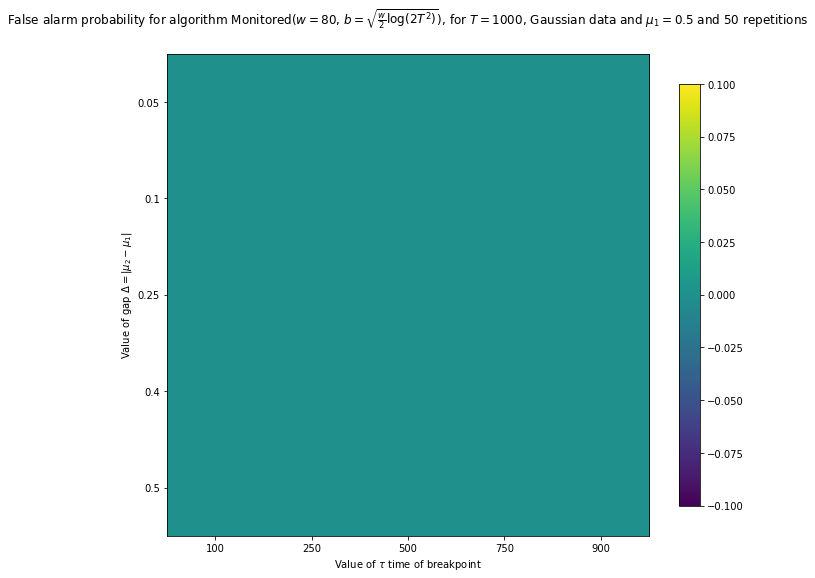
CPU times: user 2.42 s, sys: 1.1 s, total: 3.52 s
Wall time: 8.94 s
[122]:
%%time
_ = view2D_onemeasure(missed_detection, "Missed detection probability",
                      Monitored,
                      values_Delta=[0.05, 0.1, 0.25, 0.4, 0.5],
                      values_tau=[1/10, 1/4, 2/4, 3/4, 9/10],
                      firstMean=0.5,
                      horizon=1000,
                      repetitions=50,
                      gaussian=True,
                      savefig="Missed_detection_of_Monitored__Gaussian_T1000_N50__5deltas__5taus"
                     )
Exploring missed_detection for algorithm Monitored($w=80$, $b=\sqrt{\frac{w}{2} \log(2 T^2)}$) mu^1 = 0.5 and horizon = 1000...
with 5 values for Delta, and 5 values for tau, and 50 repetitions.
Saving figure with format png, to file 'Missed_detection_of_Monitored__Gaussian_T1000_N50__5deltas__5taus.png'...
       Saved! 'Missed_detection_of_Monitored__Gaussian_T1000_N50__5deltas__5taus.png' created of size '23787b', at 'Sun Dec 16 22:51:03 2018' ...
Saving figure with format pdf, to file 'Missed_detection_of_Monitored__Gaussian_T1000_N50__5deltas__5taus.pdf'...
       Saved! 'Missed_detection_of_Monitored__Gaussian_T1000_N50__5deltas__5taus.pdf' created of size '24291b', at 'Sun Dec 16 22:51:04 2018' ...
<Figure size 1425.6x777.6 with 0 Axes>
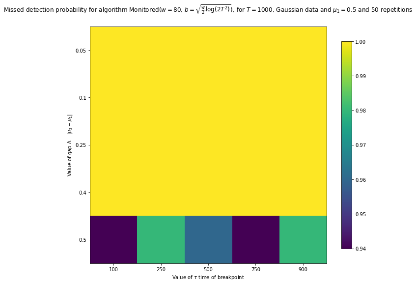
CPU times: user 2.77 s, sys: 813 ms, total: 3.58 s
Wall time: 14 s
For CUSUM
[123]:
%%time
_ = view2D_onemeasure(detection_delay, "Detection delay",
                      CUSUM,
                      values_Delta=[0.05, 0.1, 0.25, 0.4, 0.5],
                      values_tau=[1/10, 1/4, 2/4, 3/4, 9/10],
                      firstMean=0.5,
                      horizon=1000,
                      repetitions=10,
                      savefig="Detection_delay_of_CUSUM__Bernoulli_T1000_N10__5deltas__5taus",
                     )
Exploring detection_delay for algorithm CUSUM($\varepsilon=0.5$, $M=50$, $h=$'auto') mu^1 = 0.5 and horizon = 1000...
with 5 values for Delta, and 5 values for tau, and 10 repetitions.
Saving figure with format png, to file 'Detection_delay_of_CUSUM__Bernoulli_T1000_N10__5deltas__5taus.png'...
       Saved! 'Detection_delay_of_CUSUM__Bernoulli_T1000_N10__5deltas__5taus.png' created of size '23793b', at 'Sun Dec 16 22:55:04 2018' ...
Saving figure with format pdf, to file 'Detection_delay_of_CUSUM__Bernoulli_T1000_N10__5deltas__5taus.pdf'...
       Saved! 'Detection_delay_of_CUSUM__Bernoulli_T1000_N10__5deltas__5taus.pdf' created of size '24638b', at 'Sun Dec 16 22:55:05 2018' ...
<Figure size 1425.6x777.6 with 0 Axes>
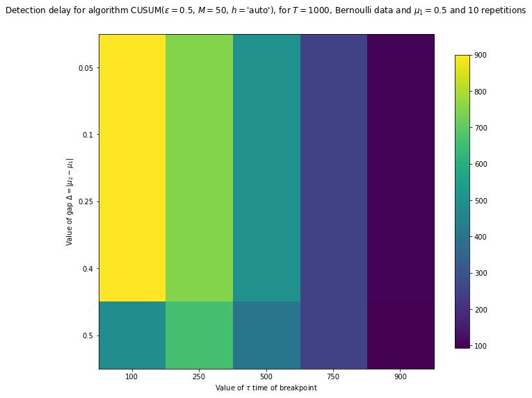
CPU times: user 2.7 s, sys: 783 ms, total: 3.48 s
Wall time: 1min 32s
[124]:
%%time
_ = view2D_onemeasure(false_alarm, "False alarm probability",
                      CUSUM,
                      values_Delta=[0.05, 0.1, 0.25, 0.4, 0.5],
                      values_tau=[1/10, 1/4, 2/4, 3/4, 9/10],
                      firstMean=0.5,
                      horizon=1000,
                      repetitions=10,
                      savefig="False_alarm_of_CUSUM__Bernoulli_T1000_N10__5deltas__5taus",
                     )
Exploring false_alarm for algorithm CUSUM($\varepsilon=0.5$, $M=50$, $h=$'auto') mu^1 = 0.5 and horizon = 1000...
with 5 values for Delta, and 5 values for tau, and 10 repetitions.
Saving figure with format png, to file 'False_alarm_of_CUSUM__Bernoulli_T1000_N10__5deltas__5taus.png'...
       Saved! 'False_alarm_of_CUSUM__Bernoulli_T1000_N10__5deltas__5taus.png' created of size '24535b', at 'Sun Dec 16 22:56:45 2018' ...
Saving figure with format pdf, to file 'False_alarm_of_CUSUM__Bernoulli_T1000_N10__5deltas__5taus.pdf'...
       Saved! 'False_alarm_of_CUSUM__Bernoulli_T1000_N10__5deltas__5taus.pdf' created of size '22776b', at 'Sun Dec 16 22:56:45 2018' ...
<Figure size 1425.6x777.6 with 0 Axes>
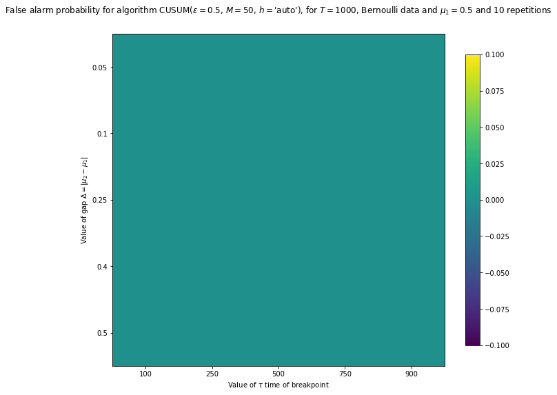
CPU times: user 2.62 s, sys: 958 ms, total: 3.58 s
Wall time: 48.4 s
[125]:
%%time
_ = view2D_onemeasure(missed_detection, "Missed detection probability",
                      CUSUM,
                      values_Delta=[0.05, 0.1, 0.25, 0.4, 0.5],
                      values_tau=[1/10, 1/4, 2/4, 3/4, 9/10],
                      firstMean=0.5,
                      horizon=1000,
                      repetitions=10,
                      savefig="Missed_detection_of_CUSUM__Bernoulli_T1000_N10__5deltas__5taus",
                     )
Exploring missed_detection for algorithm CUSUM($\varepsilon=0.5$, $M=50$, $h=$'auto') mu^1 = 0.5 and horizon = 1000...
with 5 values for Delta, and 5 values for tau, and 10 repetitions.
Saving figure with format png, to file 'Missed_detection_of_CUSUM__Bernoulli_T1000_N10__5deltas__5taus.png'...
       Saved! 'Missed_detection_of_CUSUM__Bernoulli_T1000_N10__5deltas__5taus.png' created of size '21721b', at 'Sun Dec 16 22:58:38 2018' ...
Saving figure with format pdf, to file 'Missed_detection_of_CUSUM__Bernoulli_T1000_N10__5deltas__5taus.pdf'...
       Saved! 'Missed_detection_of_CUSUM__Bernoulli_T1000_N10__5deltas__5taus.pdf' created of size '23865b', at 'Sun Dec 16 22:58:38 2018' ...
<Figure size 1425.6x777.6 with 0 Axes>
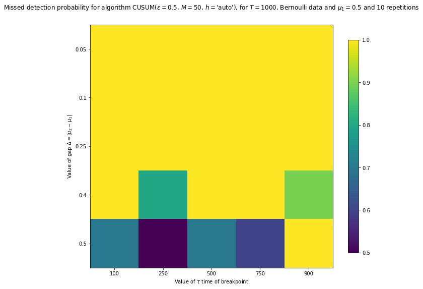
CPU times: user 2.75 s, sys: 986 ms, total: 3.74 s
Wall time: 1min 26s
Second example
[150]:
firstMean = mu_1 = 0.5
max_mu_2 = 1
nb_values_Delta = 20
min_delta = 0.15
max_delta = max_mu_2 - mu_1
epsilon = 0.03
values_Delta = np.linspace(min_delta, (1 - epsilon) * max_delta, nb_values_Delta)
print(f"Values of delta: {values_Delta}")
Values of delta: [0.15       0.16763158 0.18526316 0.20289474 0.22052632 0.23815789
 0.25578947 0.27342105 0.29105263 0.30868421 0.32631579 0.34394737
 0.36157895 0.37921053 0.39684211 0.41447368 0.43210526 0.44973684
 0.46736842 0.485     ]
[151]:
horizon = T = 1000
min_tau = 50
max_tau = T - min_tau
step = 50
values_tau = np.arange(min_tau, max_tau + 1, step)
nb_values_tau = len(values_tau)
print(f"Values of tau: {values_tau}")
Values of tau: [ 50 100 150 200 250 300 350 400 450 500 550 600 650 700 750 800 850 900
 950]
[152]:
print(f"This will give a grid of {nb_values_Delta} x {nb_values_tau} = {nb_values_Delta * nb_values_tau} values of Delta and tau to explore.")
This will give a grid of 20 x 19 = 380 values of Delta and tau to explore.
For Monitored
[153]:
%%time
_ = view2D_onemeasure(detection_delay, "Detection delay",
                      Monitored,
                      values_Delta=values_Delta,
                      values_tau=values_tau,
                      firstMean=firstMean,
                      horizon=horizon,
                      repetitions=50,
                      savefig="Detection_delay_of_CUSUM__Bernoulli_T1000_N50__20deltas__19taus",
                     )
Exploring detection_delay for algorithm Monitored($w=80$, $b=\sqrt{\frac{w}{2} \log(2 T^2)}$) mu^1 = 0.5 and horizon = 1000...
with 20 values for Delta, and 19 values for tau, and 50 repetitions.
Saving figure with format png, to file 'Detection_delay_of_CUSUM__Bernoulli_T1000_N50__20deltas__19taus.png'...
       Saved! 'Detection_delay_of_CUSUM__Bernoulli_T1000_N50__20deltas__19taus.png' created of size '35492b', at 'Mon Dec 17 00:14:07 2018' ...
Saving figure with format pdf, to file 'Detection_delay_of_CUSUM__Bernoulli_T1000_N50__20deltas__19taus.pdf'...
       Saved! 'Detection_delay_of_CUSUM__Bernoulli_T1000_N50__20deltas__19taus.pdf' created of size '26214b', at 'Mon Dec 17 00:14:07 2018' ...
<Figure size 1425.6x777.6 with 0 Axes>
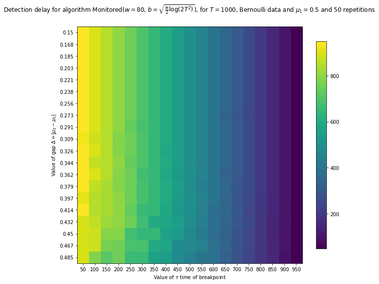
CPU times: user 18.4 s, sys: 2.3 s, total: 20.7 s
Wall time: 2min 48s
[154]:
%%time
_ = view2D_onemeasure(false_alarm, "False alarm probability",
                      Monitored,
                      values_Delta=values_Delta,
                      values_tau=values_tau,
                      firstMean=firstMean,
                      horizon=horizon,
                      repetitions=50,
                      savefig="False_alarm_of_CUSUM__Bernoulli_T1000_N50__20deltas__19taus",
                     )
Exploring false_alarm for algorithm Monitored($w=80$, $b=\sqrt{\frac{w}{2} \log(2 T^2)}$) mu^1 = 0.5 and horizon = 1000...
with 20 values for Delta, and 19 values for tau, and 50 repetitions.
Saving figure with format png, to file 'False_alarm_of_CUSUM__Bernoulli_T1000_N50__20deltas__19taus.png'...
       Saved! 'False_alarm_of_CUSUM__Bernoulli_T1000_N50__20deltas__19taus.png' created of size '36327b', at 'Mon Dec 17 00:16:36 2018' ...
Saving figure with format pdf, to file 'False_alarm_of_CUSUM__Bernoulli_T1000_N50__20deltas__19taus.pdf'...
       Saved! 'False_alarm_of_CUSUM__Bernoulli_T1000_N50__20deltas__19taus.pdf' created of size '25201b', at 'Mon Dec 17 00:16:36 2018' ...
<Figure size 1425.6x777.6 with 0 Axes>
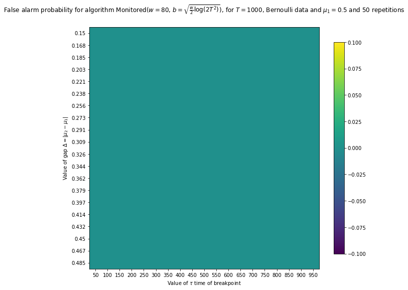
CPU times: user 18 s, sys: 2.22 s, total: 20.2 s
Wall time: 2min 29s
[155]:
%%time
_ = view2D_onemeasure(missed_detection, "Missed detection probability",
                      Monitored,
                      values_Delta=values_Delta,
                      values_tau=values_tau,
                      firstMean=firstMean,
                      horizon=horizon,
                      repetitions=50,
                      savefig="Missed_detection_of_CUSUM__Bernoulli_T1000_N50__20deltas__19taus",
                     )
Exploring missed_detection for algorithm Monitored($w=80$, $b=\sqrt{\frac{w}{2} \log(2 T^2)}$) mu^1 = 0.5 and horizon = 1000...
with 20 values for Delta, and 19 values for tau, and 50 repetitions.
Saving figure with format png, to file 'Missed_detection_of_CUSUM__Bernoulli_T1000_N50__20deltas__19taus.png'...
       Saved! 'Missed_detection_of_CUSUM__Bernoulli_T1000_N50__20deltas__19taus.png' created of size '35506b', at 'Mon Dec 17 00:19:26 2018' ...
Saving figure with format pdf, to file 'Missed_detection_of_CUSUM__Bernoulli_T1000_N50__20deltas__19taus.pdf'...
       Saved! 'Missed_detection_of_CUSUM__Bernoulli_T1000_N50__20deltas__19taus.pdf' created of size '25967b', at 'Mon Dec 17 00:19:26 2018' ...
<Figure size 1425.6x777.6 with 0 Axes>
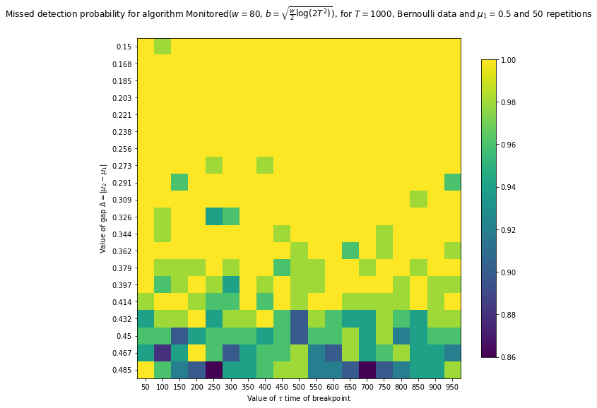
CPU times: user 19.1 s, sys: 2.27 s, total: 21.4 s
Wall time: 2min 49s
For Monitored for Gaussian data
[156]:
%%time
_ = view2D_onemeasure(detection_delay, "Detection delay",
                      Monitored,
                      values_Delta=values_Delta,
                      values_tau=values_tau,
                      firstMean=firstMean,
                      horizon=horizon,
                      repetitions=50,
                      gaussian=True,
                      savefig="Detection_delay_of_Monitored__Gaussian_T1000_N50__20deltas__19taus",
                     )
Exploring detection_delay for algorithm Monitored($w=80$, $b=\sqrt{\frac{w}{2} \log(2 T^2)}$) mu^1 = 0.5 and horizon = 1000...
with 20 values for Delta, and 19 values for tau, and 50 repetitions.
Saving figure with format png, to file 'Detection_delay_of_Monitored__Gaussian_T1000_N50__20deltas__19taus.png'...
       Saved! 'Detection_delay_of_Monitored__Gaussian_T1000_N50__20deltas__19taus.png' created of size '35101b', at 'Mon Dec 17 00:22:18 2018' ...
Saving figure with format pdf, to file 'Detection_delay_of_Monitored__Gaussian_T1000_N50__20deltas__19taus.pdf'...
       Saved! 'Detection_delay_of_Monitored__Gaussian_T1000_N50__20deltas__19taus.pdf' created of size '25794b', at 'Mon Dec 17 00:22:18 2018' ...
<Figure size 1425.6x777.6 with 0 Axes>
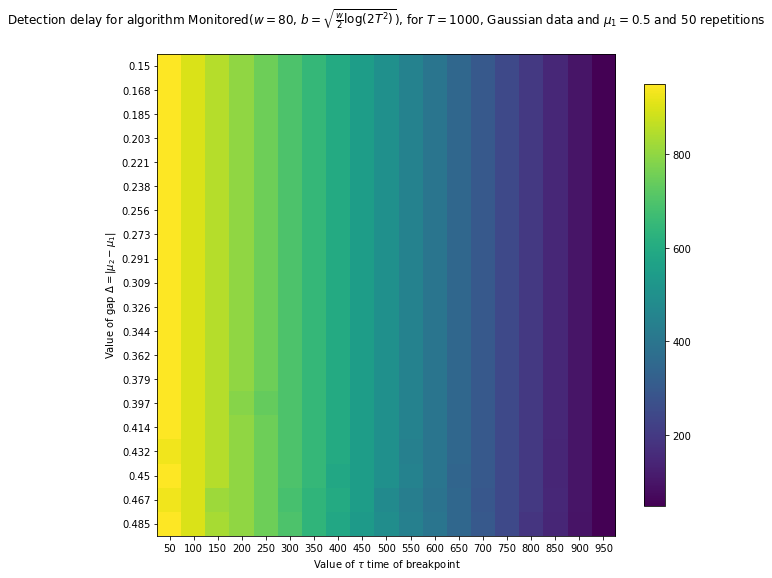
CPU times: user 18.8 s, sys: 1.76 s, total: 20.5 s
Wall time: 2min 51s
[157]:
%%time
_ = view2D_onemeasure(missed_detection, "Missed detection probability",
                      Monitored,
                      values_Delta=values_Delta,
                      values_tau=values_tau,
                      firstMean=firstMean,
                      horizon=horizon,
                      repetitions=50,
                      gaussian=True,
                      savefig="Missed_detection_of_Monitored__Gaussian_T1000_N50__20deltas__19taus",
                     )
Exploring missed_detection for algorithm Monitored($w=80$, $b=\sqrt{\frac{w}{2} \log(2 T^2)}$) mu^1 = 0.5 and horizon = 1000...
with 20 values for Delta, and 19 values for tau, and 50 repetitions.
Saving figure with format png, to file 'Missed_detection_of_Monitored__Gaussian_T1000_N50__20deltas__19taus.png'...
       Saved! 'Missed_detection_of_Monitored__Gaussian_T1000_N50__20deltas__19taus.png' created of size '34373b', at 'Mon Dec 17 00:25:19 2018' ...
Saving figure with format pdf, to file 'Missed_detection_of_Monitored__Gaussian_T1000_N50__20deltas__19taus.pdf'...
       Saved! 'Missed_detection_of_Monitored__Gaussian_T1000_N50__20deltas__19taus.pdf' created of size '25472b', at 'Mon Dec 17 00:25:19 2018' ...
<Figure size 1425.6x777.6 with 0 Axes>
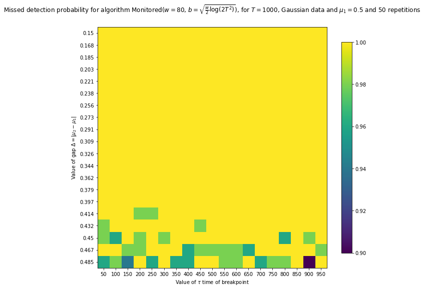
CPU times: user 19.6 s, sys: 2.16 s, total: 21.8 s
Wall time: 3min 1s
For CUSUM
[158]:
%%time
_ = view2D_onemeasure(detection_delay, "Detection delay",
                      CUSUM,
                      values_Delta=values_Delta,
                      values_tau=values_tau,
                      firstMean=firstMean,
                      horizon=horizon,
                      repetitions=10,
                      savefig="Detection_delay_of_CUSUM__Bernoulli_T1000_N10__20deltas__19taus",
                     )
Exploring detection_delay for algorithm CUSUM($\varepsilon=0.5$, $M=50$, $h=$'auto') mu^1 = 0.5 and horizon = 1000...
with 20 values for Delta, and 19 values for tau, and 10 repetitions.
Saving figure with format png, to file 'Detection_delay_of_CUSUM__Bernoulli_T1000_N10__20deltas__19taus.png'...
       Saved! 'Detection_delay_of_CUSUM__Bernoulli_T1000_N10__20deltas__19taus.png' created of size '36912b', at 'Sun Dec 16 23:05:29 2018' ...
Saving figure with format pdf, to file 'Detection_delay_of_CUSUM__Bernoulli_T1000_N10__20deltas__19taus.pdf'...
       Saved! 'Detection_delay_of_CUSUM__Bernoulli_T1000_N10__20deltas__19taus.pdf' created of size '25885b', at 'Sun Dec 16 23:05:29 2018' ...
<Figure size 1425.6x777.6 with 0 Axes>
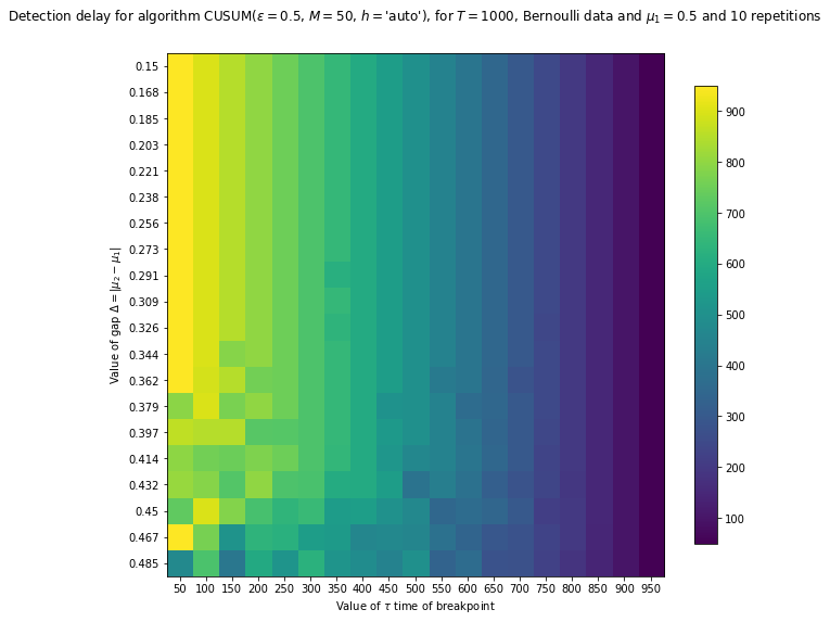
CPU times: user 23.5 s, sys: 2.69 s, total: 26.2 s
Wall time: 27min 56s
For PHT
[159]:
%%time
_ = view2D_onemeasure(detection_delay, "Detection delay",
PHT,
values_Delta=values_Delta,
values_tau=values_tau,
firstMean=firstMean,
horizon=horizon,
repetitions=5,
savefig="Detection_delay_of_PHT__Bernoulli_T1000_N5__20deltas__19taus",
)
Exploring detection_delay for algorithm PHT($\varepsilon=0.5$, $M=50$, $h=$'auto') mu^1 = 0.5 and horizon = 1000...
with 20 values for Delta, and 19 values for tau, and 5 repetitions.
Saving figure with format png, to file 'Detection_delay_of_PHT__Bernoulli_T1000_N5__20deltas__19taus.png'...
Saved! 'Detection_delay_of_PHT__Bernoulli_T1000_N5__20deltas__19taus.png' created of size '36046b', at 'Mon Dec 17 01:11:12 2018' ...
Saving figure with format pdf, to file 'Detection_delay_of_PHT__Bernoulli_T1000_N5__20deltas__19taus.pdf'...
Saved! 'Detection_delay_of_PHT__Bernoulli_T1000_N5__20deltas__19taus.pdf' created of size '24584b', at 'Mon Dec 17 01:11:12 2018' ...
<Figure size 1425.6x777.6 with 0 Axes>
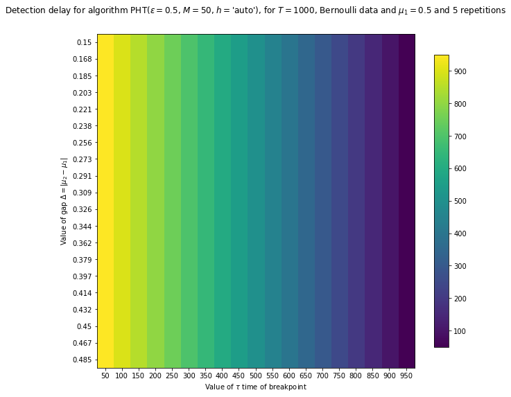
CPU times: user 18.4 s, sys: 2.27 s, total: 20.7 s
Wall time: 17min 56s
For Bernoulli GLR
[160]:
%%time
_ = view2D_onemeasure(detection_delay, "Detection delay",
BernoulliGLR,
values_Delta=values_Delta,
values_tau=values_tau,
firstMean=firstMean,
horizon=horizon,
repetitions=10,
savefig="Detection_delay_of_BernoulliGLR__Bernoulli_T1000_N10__20deltas__19taus",
)
Exploring detection_delay for algorithm Bernoulli-GLR($h_0=1$, $\delta=auto$) mu^1 = 0.5 and horizon = 1000...
with 20 values for Delta, and 19 values for tau, and 10 repetitions.
Saving figure with format png, to file 'Detection_delay_of_BernoulliGLR__Bernoulli_T1000_N10__20deltas__19taus.png'...
Saved! 'Detection_delay_of_BernoulliGLR__Bernoulli_T1000_N10__20deltas__19taus.png' created of size '35663b', at 'Mon Dec 17 02:08:22 2018' ...
Saving figure with format pdf, to file 'Detection_delay_of_BernoulliGLR__Bernoulli_T1000_N10__20deltas__19taus.pdf'...
Saved! 'Detection_delay_of_BernoulliGLR__Bernoulli_T1000_N10__20deltas__19taus.pdf' created of size '27345b', at 'Mon Dec 17 02:08:22 2018' ...
<Figure size 1425.6x777.6 with 0 Axes>
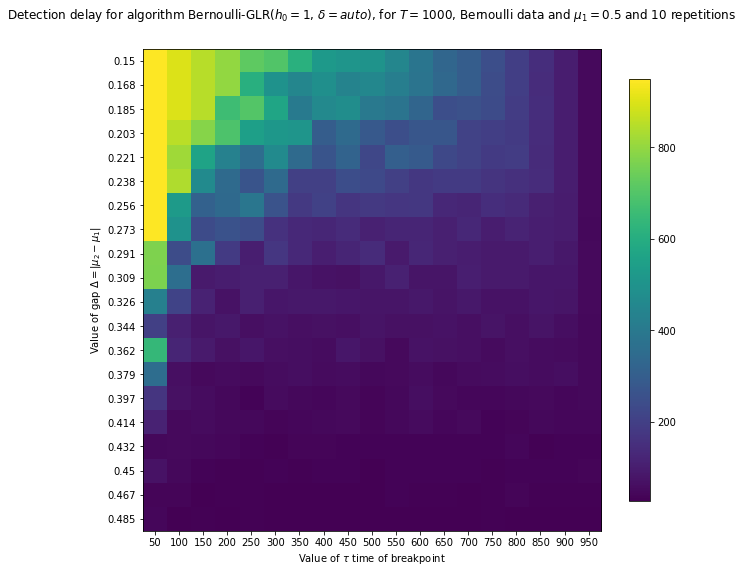
CPU times: user 23 s, sys: 2.6 s, total: 25.6 s
Wall time: 57min 10s
[161]:
%%time
_ = view2D_onemeasure(detection_delay, "Detection delay",
BernoulliGLR,
values_Delta=values_Delta,
values_tau=values_tau,
firstMean=firstMean,
horizon=horizon,
repetitions=10,
gaussian=True,
savefig="Detection_delay_of_BernoulliGLR__Gaussian_T1000_N10__20deltas__19taus",
)
Exploring detection_delay for algorithm Bernoulli-GLR($h_0=1$, $\delta=auto$) mu^1 = 0.5 and horizon = 1000...
with 20 values for Delta, and 19 values for tau, and 10 repetitions.
Saving figure with format png, to file 'Detection_delay_of_BernoulliGLR__Gaussian_T1000_N10__20deltas__19taus.png'...
Saved! 'Detection_delay_of_BernoulliGLR__Gaussian_T1000_N10__20deltas__19taus.png' created of size '35469b', at 'Mon Dec 17 03:11:46 2018' ...
Saving figure with format pdf, to file 'Detection_delay_of_BernoulliGLR__Gaussian_T1000_N10__20deltas__19taus.pdf'...
Saved! 'Detection_delay_of_BernoulliGLR__Gaussian_T1000_N10__20deltas__19taus.pdf' created of size '27169b', at 'Mon Dec 17 03:11:46 2018' ...
<Figure size 1425.6x777.6 with 0 Axes>
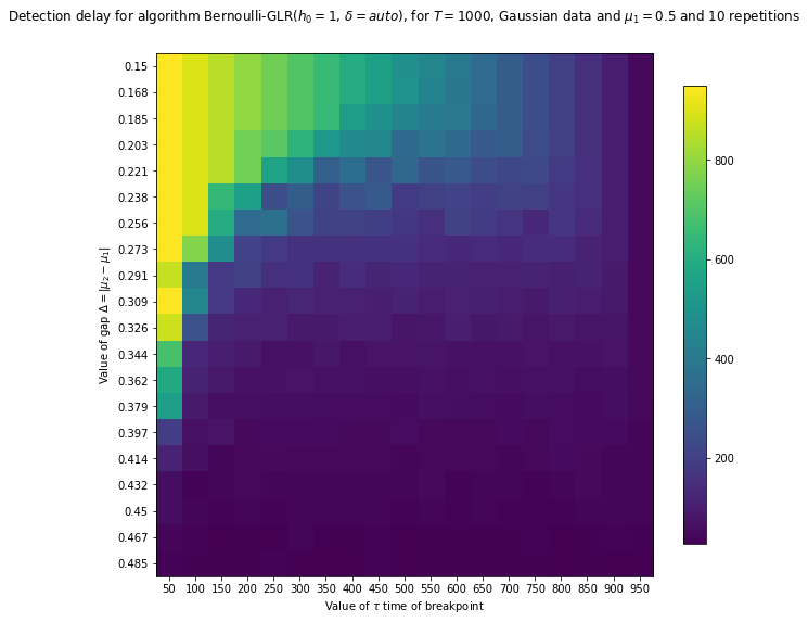
CPU times: user 23.1 s, sys: 2.66 s, total: 25.7 s
Wall time: 1h 3min 24s
For Gaussian GLR
[162]:
%%time
_ = view2D_onemeasure(detection_delay, "Detection delay",
GaussianGLR,
values_Delta=values_Delta,
values_tau=values_tau,
firstMean=firstMean,
horizon=horizon,
repetitions=10,
savefig="Detection_delay_of_GaussianGLR__Bernoulli_T1000_N10__20deltas__19taus",
)
Exploring detection_delay for algorithm Gaussian-GLR($h_0=1$, $\delta=auto$) mu^1 = 0.5 and horizon = 1000...
with 20 values for Delta, and 19 values for tau, and 10 repetitions.
Saving figure with format png, to file 'Detection_delay_of_GaussianGLR__Bernoulli_T1000_N10__20deltas__19taus.png'...
Saved! 'Detection_delay_of_GaussianGLR__Bernoulli_T1000_N10__20deltas__19taus.png' created of size '35772b', at 'Mon Dec 17 03:38:44 2018' ...
Saving figure with format pdf, to file 'Detection_delay_of_GaussianGLR__Bernoulli_T1000_N10__20deltas__19taus.pdf'...
Saved! 'Detection_delay_of_GaussianGLR__Bernoulli_T1000_N10__20deltas__19taus.pdf' created of size '27383b', at 'Mon Dec 17 03:38:45 2018' ...
<Figure size 1425.6x777.6 with 0 Axes>
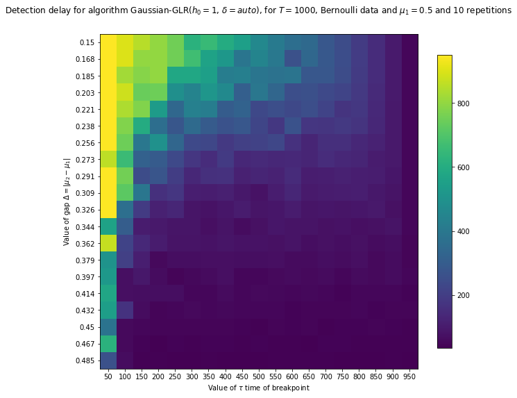
CPU times: user 22.3 s, sys: 2.51 s, total: 24.8 s
Wall time: 26min 58s
[163]:
%%time
_ = view2D_onemeasure(detection_delay, "Detection delay",
GaussianGLR,
values_Delta=values_Delta,
values_tau=values_tau,
firstMean=firstMean,
horizon=horizon,
repetitions=1,
gaussian=True,
savefig="Detection_delay_of_GaussianGLR__Gaussian_T1000_N1__20deltas__19taus",
)
Exploring detection_delay for algorithm Gaussian-GLR($h_0=1$, $\delta=auto$) mu^1 = 0.5 and horizon = 1000...
with 20 values for Delta, and 19 values for tau, and 1 repetitions.
Saving figure with format png, to file 'Detection_delay_of_GaussianGLR__Gaussian_T1000_N1__20deltas__19taus.png'...
Saved! 'Detection_delay_of_GaussianGLR__Gaussian_T1000_N1__20deltas__19taus.png' created of size '35440b', at 'Mon Dec 17 03:41:50 2018' ...
Saving figure with format pdf, to file 'Detection_delay_of_GaussianGLR__Gaussian_T1000_N1__20deltas__19taus.pdf'...
Saved! 'Detection_delay_of_GaussianGLR__Gaussian_T1000_N1__20deltas__19taus.pdf' created of size '26984b', at 'Mon Dec 17 03:41:50 2018' ...
<Figure size 1425.6x777.6 with 0 Axes>
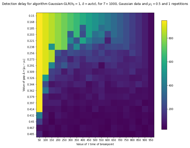
CPU times: user 14.5 s, sys: 1.86 s, total: 16.4 s
Wall time: 3min 5s
For Sub-Gaussian GLR
[164]:
%%time
_ = view2D_onemeasure(detection_delay, "Detection delay",
SubGaussianGLR,
values_Delta=values_Delta,
values_tau=values_tau,
firstMean=firstMean,
horizon=horizon,
repetitions=10,
savefig="Detection_delay_of_SubGaussianGLR__Bernoulli_T1000_N10__20deltas__19taus",
)
Exploring detection_delay for algorithm SubGaussian-GLR($\delta=$0.01, $\sigma=$0.25, joint) mu^1 = 0.5 and horizon = 1000...
with 20 values for Delta, and 19 values for tau, and 1 repetitions.
Saving figure with format png, to file 'Detection_delay_of_SubGaussianGLR__Bernoulli_T1000_N1__20deltas__19taus.png'...
Saved! 'Detection_delay_of_SubGaussianGLR__Bernoulli_T1000_N1__20deltas__19taus.png' created of size '36307b', at 'Mon Dec 17 03:42:14 2018' ...
Saving figure with format pdf, to file 'Detection_delay_of_SubGaussianGLR__Bernoulli_T1000_N1__20deltas__19taus.pdf'...
Saved! 'Detection_delay_of_SubGaussianGLR__Bernoulli_T1000_N1__20deltas__19taus.pdf' created of size '27239b', at 'Mon Dec 17 03:42:14 2018' ...
<Figure size 1425.6x777.6 with 0 Axes>
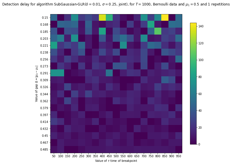
CPU times: user 13.6 s, sys: 1.75 s, total: 15.3 s
Wall time: 24.1 s
[165]:
%%time
_ = view2D_onemeasure(false_alarm, "False alarm",
SubGaussianGLR,
values_Delta=values_Delta,
values_tau=values_tau,
firstMean=firstMean,
horizon=horizon,
repetitions=10,
savefig="False_alarm__SubGaussianGLR__Bernoulli_T1000_N10__20deltas__19taus",
)
Exploring false_alarm for algorithm SubGaussian-GLR($\delta=$0.01, $\sigma=$0.25, joint) mu^1 = 0.5 and horizon = 1000...
with 20 values for Delta, and 19 values for tau, and 1 repetitions.
Saving figure with format png, to file 'False_alarm__SubGaussianGLR__Bernoulli_T1000_N1__20deltas__19taus.png'...
Saved! 'False_alarm__SubGaussianGLR__Bernoulli_T1000_N1__20deltas__19taus.png' created of size '32667b', at 'Mon Dec 17 03:42:30 2018' ...
Saving figure with format pdf, to file 'False_alarm__SubGaussianGLR__Bernoulli_T1000_N1__20deltas__19taus.pdf'...
Saved! 'False_alarm__SubGaussianGLR__Bernoulli_T1000_N1__20deltas__19taus.pdf' created of size '24694b', at 'Mon Dec 17 03:42:30 2018' ...
<Figure size 1425.6x777.6 with 0 Axes>
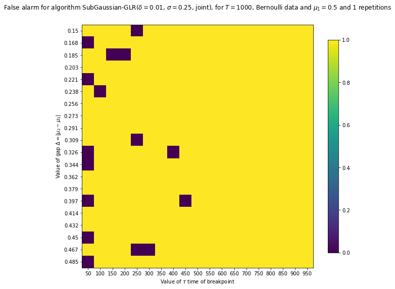
CPU times: user 13.1 s, sys: 1.69 s, total: 14.8 s
Wall time: 16 s
With this tuning (\(\delta=0.01\)), the Sub-Gaussian GLR almost always gives a false alarm! It detects too soon!
For Gaussian data:
[166]:
%%time
_ = view2D_onemeasure(detection_delay, "Detection delay",
SubGaussianGLR,
values_Delta=values_Delta,
values_tau=values_tau,
firstMean=firstMean,
horizon=horizon,
repetitions=10,
gaussian=True,
savefig="Detection_delay__SubGaussianGLR__Gaussian_T1000_N10__20deltas__19taus",
)
Exploring detection_delay for algorithm SubGaussian-GLR($\delta=$0.01, $\sigma=$0.25, joint) mu^1 = 0.5 and horizon = 1000...
with 20 values for Delta, and 19 values for tau, and 1 repetitions.
Saving figure with format png, to file 'Detection_delay__SubGaussianGLR__Gaussian_T1000_N1__20deltas__19taus.png'...
Saved! 'Detection_delay__SubGaussianGLR__Gaussian_T1000_N1__20deltas__19taus.png' created of size '35279b', at 'Mon Dec 17 03:43:13 2018' ...
Saving figure with format pdf, to file 'Detection_delay__SubGaussianGLR__Gaussian_T1000_N1__20deltas__19taus.pdf'...
Saved! 'Detection_delay__SubGaussianGLR__Gaussian_T1000_N1__20deltas__19taus.pdf' created of size '26175b', at 'Mon Dec 17 03:43:13 2018' ...
<Figure size 1425.6x777.6 with 0 Axes>
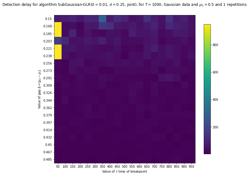
CPU times: user 14.1 s, sys: 1.64 s, total: 15.8 s
Wall time: 43.3 s
[167]:
%%time
_ = view2D_onemeasure(false_alarm, "False alarm",
SubGaussianGLR,
values_Delta=values_Delta,
values_tau=values_tau,
firstMean=firstMean,
horizon=horizon,
repetitions=1,
gaussian=True,
savefig="False_alarm__SubGaussianGLR__Gaussian_T1000_N1__20deltas__19taus",
)
Exploring false_alarm for algorithm SubGaussian-GLR($\delta=$0.01, $\sigma=$0.25, joint) mu^1 = 0.5 and horizon = 1000...
with 20 values for Delta, and 19 values for tau, and 1 repetitions.
Saving figure with format png, to file 'False_alarm__SubGaussianGLR__Gaussian_T1000_N1__20deltas__19taus.png'...
Saved! 'False_alarm__SubGaussianGLR__Gaussian_T1000_N1__20deltas__19taus.png' created of size '35218b', at 'Mon Dec 17 03:47:38 2018' ...
Saving figure with format pdf, to file 'False_alarm__SubGaussianGLR__Gaussian_T1000_N1__20deltas__19taus.pdf'...
Saved! 'False_alarm__SubGaussianGLR__Gaussian_T1000_N1__20deltas__19taus.pdf' created of size '24203b', at 'Mon Dec 17 03:47:38 2018' ...
<Figure size 1425.6x777.6 with 0 Axes>
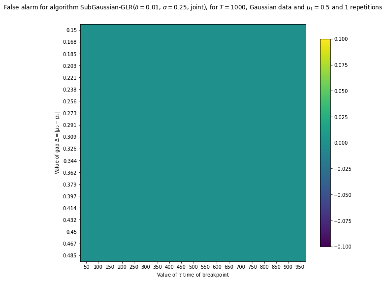
CPU times: user 14.7 s, sys: 1.87 s, total: 16.6 s
Wall time: 4min 25s
For another, simpler problem.
[168]:
horizon = T = 200
min_tau = 10
max_tau = T - min_tau
step = 10
values_tau = np.arange(min_tau, max_tau + 1, step)
nb_values_tau = len(values_tau)
print(f"Values of tau: {values_tau}")
Values of tau: [ 10 20 30 40 50 60 70 80 90 100 110 120 130 140 150 160 170 180
190]
[169]:
firstMean = mu_1 = -1.0
max_mu_2 = 1.0
nb_values_Delta = nb_values_tau
max_delta = max_mu_2 - mu_1
epsilon = 0.01
values_Delta = np.linspace(epsilon * max_delta, (1 - epsilon) * max_delta, nb_values_Delta)
print(f"Values of delta: {values_Delta}")
Values of delta: [0.02 0.12888889 0.23777778 0.34666667 0.45555556 0.56444444
0.67333333 0.78222222 0.89111111 1. 1.10888889 1.21777778
1.32666667 1.43555556 1.54444444 1.65333333 1.76222222 1.87111111
1.98 ]
[170]:
print(f"This will give a grid of {nb_values_Delta} x {nb_values_tau} = {nb_values_Delta * nb_values_tau} values of Delta and tau to explore.")
This will give a grid of 19 x 19 = 361 values of Delta and tau to explore.
[171]:
%%time
_ = view2D_onemeasure(detection_delay, "Detection delay",
SubGaussianGLR,
values_Delta=values_Delta,
values_tau=values_tau,
firstMean=firstMean,
horizon=horizon,
repetitions=10,
gaussian=True,
savefig="Detection_delay__SubGaussianGLR__Gaussian_T1000_N10__19deltas__19taus",
)
Exploring detection_delay for algorithm SubGaussian-GLR($\delta=$0.01, $\sigma=$0.25, joint) mu^1 = -1.0 and horizon = 200...
with 19 values for Delta, and 19 values for tau, and 10 repetitions.
Saving figure with format png, to file 'Detection_delay__SubGaussianGLR__Gaussian_T1000_N10__19deltas__19taus.png'...
Saved! 'Detection_delay__SubGaussianGLR__Gaussian_T1000_N10__19deltas__19taus.png' created of size '33365b', at 'Mon Dec 17 03:48:25 2018' ...
Saving figure with format pdf, to file 'Detection_delay__SubGaussianGLR__Gaussian_T1000_N10__19deltas__19taus.pdf'...
Saved! 'Detection_delay__SubGaussianGLR__Gaussian_T1000_N10__19deltas__19taus.pdf' created of size '25840b', at 'Mon Dec 17 03:48:25 2018' ...
<Figure size 1425.6x777.6 with 0 Axes>
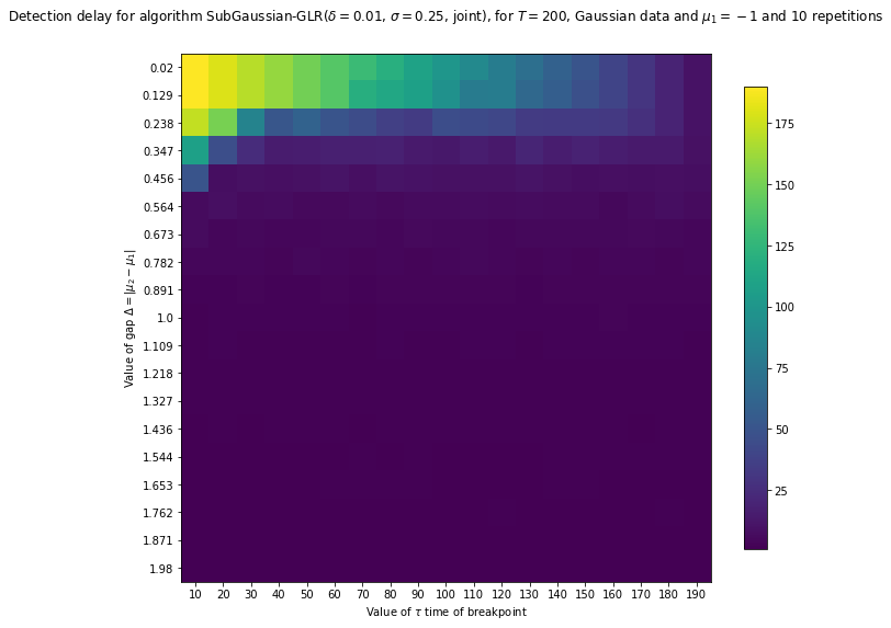
CPU times: user 13.6 s, sys: 1.58 s, total: 15.1 s
Wall time: 46.9 s
[172]:
%%time
_ = view2D_onemeasure(false_alarm, "False alarm probability",
SubGaussianGLR,
values_Delta=values_Delta,
values_tau=values_tau,
firstMean=firstMean,
horizon=horizon,
repetitions=10,
gaussian=True,
savefig="False_alarm__SubGaussianGLR__Gaussian_T1000_N10__19deltas__19taus",
)
Exploring false_alarm for algorithm SubGaussian-GLR($\delta=$0.01, $\sigma=$0.25, joint) mu^1 = -1.0 and horizon = 200...
with 19 values for Delta, and 19 values for tau, and 10 repetitions.
Saving figure with format png, to file 'False_alarm__SubGaussianGLR__Gaussian_T1000_N10__19deltas__19taus.png'...
Saved! 'False_alarm__SubGaussianGLR__Gaussian_T1000_N10__19deltas__19taus.png' created of size '32154b', at 'Mon Dec 17 03:50:09 2018' ...
Saving figure with format pdf, to file 'False_alarm__SubGaussianGLR__Gaussian_T1000_N10__19deltas__19taus.pdf'...
Saved! 'False_alarm__SubGaussianGLR__Gaussian_T1000_N10__19deltas__19taus.pdf' created of size '24634b', at 'Mon Dec 17 03:50:09 2018' ...
<Figure size 1425.6x777.6 with 0 Axes>
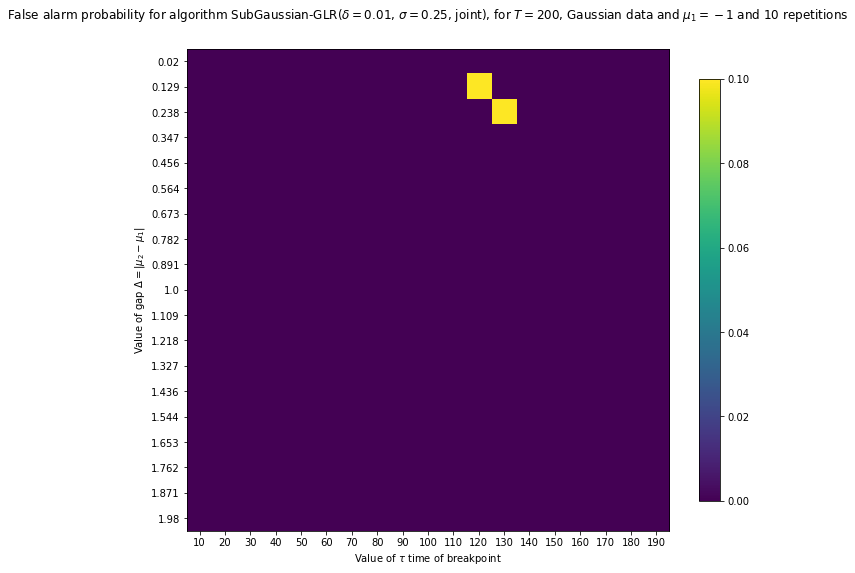
CPU times: user 15 s, sys: 1.78 s, total: 16.7 s
Wall time: 1min 44s
[173]:
%%time
_ = view2D_onemeasure(missed_detection, "Missed detection probability",
SubGaussianGLR,
values_Delta=values_Delta,
values_tau=values_tau,
firstMean=firstMean,
horizon=horizon,
repetitions=10,
gaussian=True,
savefig="Missed_detection__SubGaussianGLR__Gaussian_T1000_N10__19deltas__19taus",
)
Exploring missed_detection for algorithm SubGaussian-GLR($\delta=$0.01, $\sigma=$0.25, joint) mu^1 = -1.0 and horizon = 200...
with 19 values for Delta, and 19 values for tau, and 10 repetitions.
Saving figure with format png, to file 'Missed_detection__SubGaussianGLR__Gaussian_T1000_N10__19deltas__19taus.png'...
Saved! 'Missed_detection__SubGaussianGLR__Gaussian_T1000_N10__19deltas__19taus.png' created of size '31890b', at 'Mon Dec 17 03:50:57 2018' ...
Saving figure with format pdf, to file 'Missed_detection__SubGaussianGLR__Gaussian_T1000_N10__19deltas__19taus.pdf'...
Saved! 'Missed_detection__SubGaussianGLR__Gaussian_T1000_N10__19deltas__19taus.pdf' created of size '25184b', at 'Mon Dec 17 03:50:57 2018' ...
<Figure size 1425.6x777.6 with 0 Axes>
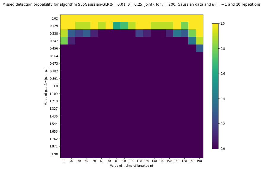
CPU times: user 13.3 s, sys: 1.81 s, total: 15.1 s
Wall time: 47.3 s
Exploring the parameters of change point detection algorithms: how to tune them?
A simple problem function
We consider again a problem with \(T=1000\) samples, first coming from a distribution of mean \(\mu^1 = 0.25\) then from a second distribution of mean \(\mu^2 = 0.75\) (largest gap, \(\Delta = 0.5\)). We consider also a single breakpoint located at \(\tau = \frac{1}{2} T = 500\), ie the algorithm will observe \(500\) samples from \(\nu^1\) then \(500\) from \(\nu^2\).
We can consider Bernoulli or Gaussian distributions.
[241]:
horizon = 200
firstMean = mu_1 = 0.25
secondMean = mu_2 = 0.75
gap = mu_2 - mu_1
tau = 0.5
A generic function
[242]:
def explore_parameters(measure,
CDAlgorithm,
tau=tau,
firstMean=mu_1,
secondMean=mu_2,
horizon=horizon,
repetitions=10,
verbose=True,
gaussian=False,
n_jobs=1,
list_of_args_kwargs=tuple(),
mean=True,
):
if isinstance(tau, float): tau = int(tau * horizon)
print(f"\nExploring {measure.__name__} for algorithm {CDAlgorithm}, mu^1 = {firstMean}, mu^2 = {secondMean}, and horizon = {horizon}, tau = {tau}...")
nb_of_args_kwargs = len(list_of_args_kwargs)
print(f"with {nb_of_args_kwargs} values for args, kwargs, and {repetitions} repetitions.")
results = np.zeros(nb_of_args_kwargs) if mean else np.zeros((repetitions, nb_of_args_kwargs))
for i, argskwargs in tqdm(enumerate(list_of_args_kwargs), desc="ArgsKwargs", leave=False):
args, kwargs = argskwargs
# now the random Monte Carlo repetitions
for j, rep in tqdm(enumerate(range(repetitions)), desc="Repetitions", leave=False):
data = get_toy_data(firstMean=firstMean, secondMean=secondMean, tau=tau, horizon=horizon, gaussian=gaussian)
result = measure(data, tau, CDAlgorithm, *args, **kwargs)
if mean:
results[i] += result
else:
results[j, i] = result
if mean:
results[i] /= repetitions
if verbose: print(f"For args = {args}, kwargs = {kwargs} ({i}th), {'mean' if mean else 'vector of'} result = {results[i]}")
return results
I want to (try to) use `joblib.Parallel <https://joblib.readthedocs.io/en/latest/parallel.html>`__ to run the “repetitions” for loop in parallel, for instance on 4 cores on my machine.
[243]:
def explore_parameters_parallel(measure,
CDAlgorithm,
tau=tau,
firstMean=mu_1,
secondMean=mu_2,
horizon=horizon,
repetitions=10,
verbose=True,
gaussian=False,
n_jobs=CPU_COUNT,
list_of_args_kwargs=tuple(),
mean=True,
):
if isinstance(tau, float): tau = int(tau * horizon)
print(f"\nExploring {measure.__name__} for algorithm {CDAlgorithm}, mu^1 = {firstMean}, mu^2 = {secondMean}, and horizon = {horizon}, tau = {tau}...")
nb_of_args_kwargs = len(list_of_args_kwargs)
print(f"with {nb_of_args_kwargs} values for args, kwargs, and {repetitions} repetitions.")
results = np.zeros(nb_of_args_kwargs) if mean else np.zeros((repetitions, nb_of_args_kwargs))
def delayed_measure(i, j, argskwargs):
args, kwargs = argskwargs
data = get_toy_data(firstMean=firstMean, secondMean=secondMean, tau=tau, horizon=horizon, gaussian=gaussian)
return i, j, measure(data, tau, CDAlgorithm, *args, **kwargs)
# now the random Monte Carlo repetitions
for i, j, result in Parallel(n_jobs=n_jobs, verbose=int(verbose))(
delayed(delayed_measure)(i, j, argskwargs)
for i, argskwargs in tqdm(enumerate(list_of_args_kwargs), desc="ArgsKwargs", leave=False)
for j, rep in tqdm(enumerate(range(repetitions)), desc="Repetitions||", leave=False)
):
if mean:
results[i] += result
else:
results[j, i] = result
if mean:
results /= repetitions
if verbose:
for i, argskwargs in enumerate(list_of_args_kwargs):
args, kwargs = argskwargs
print(f"For args = {args}, kwargs = {kwargs} ({i}th), {'mean' if mean else 'vector of'} result = {results[i]}")
return results
Plotting the result as a 1D plot
[244]:
def view1D_explore_parameters(measure, name,
CDAlgorithm,
tau=tau,
firstMean=mu_1,
secondMean=mu_2,
horizon=horizon,
repetitions=10,
verbose=False,
gaussian=False,
n_jobs=CPU_COUNT,
list_of_args_kwargs=tuple(),
argskwargs2str=None,
savefig=None,
):
explore = explore_parameters_parallel if n_jobs > 1 else explore_parameters
results = explore(measure,
CDAlgorithm,
tau=tau,
firstMean=mu_1,
secondMean=mu_2,
horizon=horizon,
repetitions=repetitions,
verbose=verbose,
gaussian=gaussian,
n_jobs=n_jobs,
list_of_args_kwargs=list_of_args_kwargs,
mean=False,
)
fig = plt.figure()
plt.boxplot(results)
plt.title(fr"{name} for {CDAlgorithm.__name__}, for $T={horizon}$, {'Gaussian' if gaussian else 'Bernoulli'} data, and $\mu_1={firstMean:.3g}$, $\mu_2={secondMean:.3g}$, $\tau={tau:.3g}$ and ${repetitions}$ repetitions")
plt.ylabel(f"{name}")
x_ticklabels = []
for argskwargs in list_of_args_kwargs:
args, kwargs = argskwargs
x_ticklabels.append(f"{args}, {kwargs}" if argskwargs2str is None else argskwargs2str(args, kwargs))
ax = plt.gca()
ax.set_xticklabels(x_ticklabels, rotation=80, verticalalignment="top")
show_and_save(savefig=savefig)
return fig
Experiments for Monitored
[245]:
list_of_args_kwargs_for_Monitored = tuple([
((), {'window_size': w, 'threshold_b': None}) # empty args, kwargs = {window_size=80, threshold_b=None}
for w in [5, 10, 20, 40, 80, 120, 160, 200, 250, 300, 350, 400, 500, 1000, 1500]
])
[246]:
argskwargs2str_for_Monitored = lambda args, kwargs: fr"$w={kwargs['window_size']:.4g}$"
On a first Bernoulli problem, a very easy one (with a large gap of \(\Delta=0.5\)).
[247]:
horizon = 100
firstMean = mu_1 = 0.25
secondMean = mu_2 = 0.75
gap = mu_2 - mu_1
tau = 0.5
[373]:
%%time
explore_parameters(detection_delay,
Monitored,
tau=tau,
firstMean=mu_1,
secondMean=mu_2,
horizon=horizon,
repetitions=10,
verbose=True,
gaussian=False,
n_jobs=1,
list_of_args_kwargs=list_of_args_kwargs_for_Monitored,
)
Exploring detection_delay for algorithm <class '__main__.Monitored'>, mu^1 = 0.25, mu^2 = 0.75, and horizon = 100, tau = 50...
with 15 values for args, kwargs, and 10 repetitions.
For args = (), kwargs = {'window_size': 5, 'threshold_b': None} (0th), mean result = 50.0
For args = (), kwargs = {'window_size': 10, 'threshold_b': None} (1th), mean result = 50.0
For args = (), kwargs = {'window_size': 20, 'threshold_b': None} (2th), mean result = 50.0
For args = (), kwargs = {'window_size': 40, 'threshold_b': None} (3th), mean result = 50.0
For args = (), kwargs = {'window_size': 80, 'threshold_b': None} (4th), mean result = 37.9
For args = (), kwargs = {'window_size': 120, 'threshold_b': None} (5th), mean result = 50.0
For args = (), kwargs = {'window_size': 160, 'threshold_b': None} (6th), mean result = 50.0
For args = (), kwargs = {'window_size': 200, 'threshold_b': None} (7th), mean result = 50.0
For args = (), kwargs = {'window_size': 250, 'threshold_b': None} (8th), mean result = 50.0
For args = (), kwargs = {'window_size': 300, 'threshold_b': None} (9th), mean result = 50.0
For args = (), kwargs = {'window_size': 350, 'threshold_b': None} (10th), mean result = 50.0
For args = (), kwargs = {'window_size': 400, 'threshold_b': None} (11th), mean result = 50.0
For args = (), kwargs = {'window_size': 500, 'threshold_b': None} (12th), mean result = 50.0
For args = (), kwargs = {'window_size': 1000, 'threshold_b': None} (13th), mean result = 50.0
For args = (), kwargs = {'window_size': 1500, 'threshold_b': None} (14th), mean result = 50.0
CPU times: user 792 ms, sys: 24.9 ms, total: 817 ms
Wall time: 1.01 s
[373]:
array([50. , 50. , 50. , 50. , 37.9, 50. , 50. , 50. , 50. , 50. , 50. ,
50. , 50. , 50. , 50. ])
[374]:
%%time
explore_parameters_parallel(detection_delay,
Monitored,
tau=tau,
firstMean=mu_1,
secondMean=mu_2,
horizon=horizon,
repetitions=10,
verbose=True,
gaussian=False,
n_jobs=4,
list_of_args_kwargs=list_of_args_kwargs_for_Monitored,
)
Exploring detection_delay for algorithm <class '__main__.Monitored'>, mu^1 = 0.25, mu^2 = 0.75, and horizon = 100, tau = 50...
with 15 values for args, kwargs, and 10 repetitions.
[Parallel(n_jobs=4)]: Using backend LokyBackend with 4 concurrent workers.
For args = (), kwargs = {'window_size': 5, 'threshold_b': None} (0th), mean result = 50.0
For args = (), kwargs = {'window_size': 10, 'threshold_b': None} (1th), mean result = 50.0
For args = (), kwargs = {'window_size': 20, 'threshold_b': None} (2th), mean result = 50.0
For args = (), kwargs = {'window_size': 40, 'threshold_b': None} (3th), mean result = 50.0
For args = (), kwargs = {'window_size': 80, 'threshold_b': None} (4th), mean result = 38.9
For args = (), kwargs = {'window_size': 120, 'threshold_b': None} (5th), mean result = 50.0
For args = (), kwargs = {'window_size': 160, 'threshold_b': None} (6th), mean result = 50.0
For args = (), kwargs = {'window_size': 200, 'threshold_b': None} (7th), mean result = 50.0
For args = (), kwargs = {'window_size': 250, 'threshold_b': None} (8th), mean result = 50.0
For args = (), kwargs = {'window_size': 300, 'threshold_b': None} (9th), mean result = 50.0
For args = (), kwargs = {'window_size': 350, 'threshold_b': None} (10th), mean result = 50.0
For args = (), kwargs = {'window_size': 400, 'threshold_b': None} (11th), mean result = 50.0
For args = (), kwargs = {'window_size': 500, 'threshold_b': None} (12th), mean result = 50.0
For args = (), kwargs = {'window_size': 1000, 'threshold_b': None} (13th), mean result = 50.0
For args = (), kwargs = {'window_size': 1500, 'threshold_b': None} (14th), mean result = 50.0
CPU times: user 619 ms, sys: 139 ms, total: 758 ms
Wall time: 1.87 s
[Parallel(n_jobs=4)]: Done 150 out of 150 | elapsed: 1.8s finished
[374]:
array([50. , 50. , 50. , 50. , 38.9, 50. , 50. , 50. , 50. , 50. , 50. ,
50. , 50. , 50. , 50. ])
[375]:
%%time
_ = view1D_explore_parameters(detection_delay, "Detection delay",
Monitored,
tau=tau,
firstMean=mu_1,
secondMean=mu_2,
horizon=horizon,
repetitions=100,
gaussian=False,
n_jobs=4,
list_of_args_kwargs=list_of_args_kwargs_for_Monitored,
argskwargs2str=argskwargs2str_for_Monitored,
savefig=f"Detection_delay__Monitored__Bernoulli_T1000_N100__{len(list_of_args_kwargs_for_Monitored)}",
)
Exploring detection_delay for algorithm <class '__main__.Monitored'>, mu^1 = 0.25, mu^2 = 0.75, and horizon = 100, tau = 50...
with 15 values for args, kwargs, and 100 repetitions.
Saving figure with format png, to file 'Detection_delay__Monitored__Bernoulli_T1000_N100__15.png'...
Saved! 'Detection_delay__Monitored__Bernoulli_T1000_N100__15.png' created of size '25734b', at 'Mon Dec 17 13:13:36 2018' ...
Saving figure with format pdf, to file 'Detection_delay__Monitored__Bernoulli_T1000_N100__15.pdf'...
Saved! 'Detection_delay__Monitored__Bernoulli_T1000_N100__15.pdf' created of size '17219b', at 'Mon Dec 17 13:13:36 2018' ...
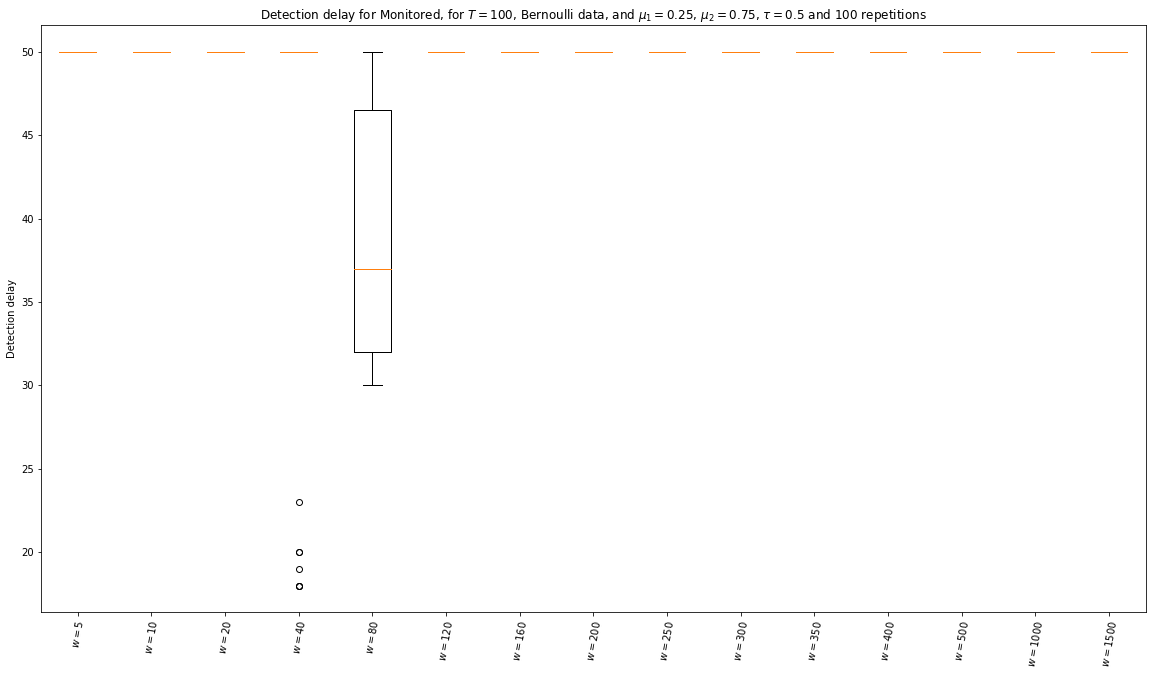
CPU times: user 2.36 s, sys: 536 ms, total: 2.89 s
Wall time: 4.07 s
On the same problem, with \(10000\) data instead of \(1000\).
[376]:
%%time
_ = view1D_explore_parameters(detection_delay, "Detection delay",
Monitored,
tau=tau,
firstMean=mu_1,
secondMean=mu_2,
horizon=10*horizon,
repetitions=100,
gaussian=False,
n_jobs=4,
list_of_args_kwargs=list_of_args_kwargs_for_Monitored,
argskwargs2str=argskwargs2str_for_Monitored,
savefig=f"Detection_delay__Monitored__Bernoulli_T10000_N100__{len(list_of_args_kwargs_for_Monitored)}",
)
Exploring detection_delay for algorithm <class '__main__.Monitored'>, mu^1 = 0.25, mu^2 = 0.75, and horizon = 1000, tau = 500...
with 15 values for args, kwargs, and 100 repetitions.
Saving figure with format png, to file 'Detection_delay__Monitored__Bernoulli_T10000_N100__15.png'...
Saved! 'Detection_delay__Monitored__Bernoulli_T10000_N100__15.png' created of size '27448b', at 'Mon Dec 17 13:13:47 2018' ...
Saving figure with format pdf, to file 'Detection_delay__Monitored__Bernoulli_T10000_N100__15.pdf'...
Saved! 'Detection_delay__Monitored__Bernoulli_T10000_N100__15.pdf' created of size '19215b', at 'Mon Dec 17 13:13:47 2018' ...
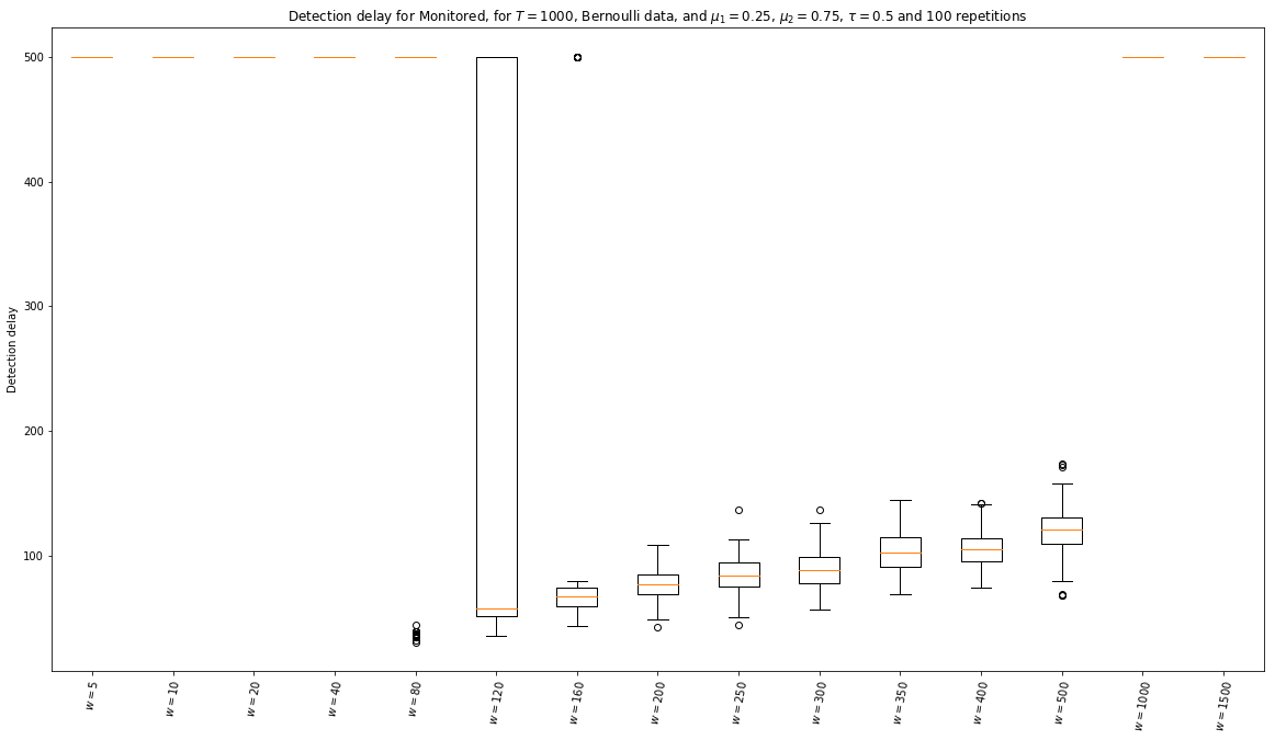
CPU times: user 2.31 s, sys: 737 ms, total: 3.04 s
Wall time: 10.8 s
On two Gaussian problems, one with a gap of \(\Delta=0.5\) (easy) and a harder with a gap of \(\Delta=0.1\). It is very intriguing that small difference in the gap can yield such large differences in the detection delay (or missed detection probability, as having a detection delay of \(D=T-\tau\) means a missed detection!).
[377]:
horizon = 10000
firstMean = mu_1 = -0.25
secondMean = mu_2 = 0.25
gap = mu_2 - mu_1
tau = 0.5
[378]:
%%time
_ = view1D_explore_parameters(detection_delay, "Detection delay",
Monitored,
tau=tau,
firstMean=mu_1,
secondMean=mu_2,
horizon=horizon,
repetitions=100,
gaussian=True,
n_jobs=4,
list_of_args_kwargs=list_of_args_kwargs_for_Monitored,
argskwargs2str=argskwargs2str_for_Monitored,
savefig=f"Detection_delay__Monitored__Gaussian_T1000_N100__{len(list_of_args_kwargs_for_Monitored)}",
)
Exploring detection_delay for algorithm <class '__main__.Monitored'>, mu^1 = -0.25, mu^2 = 0.25, and horizon = 10000, tau = 5000...
with 15 values for args, kwargs, and 100 repetitions.
Saving figure with format png, to file 'Detection_delay__Monitored__Gaussian_T1000_N100__15.png'...
Saved! 'Detection_delay__Monitored__Gaussian_T1000_N100__15.png' created of size '26971b', at 'Mon Dec 17 13:14:57 2018' ...
Saving figure with format pdf, to file 'Detection_delay__Monitored__Gaussian_T1000_N100__15.pdf'...
Saved! 'Detection_delay__Monitored__Gaussian_T1000_N100__15.pdf' created of size '18588b', at 'Mon Dec 17 13:14:57 2018' ...
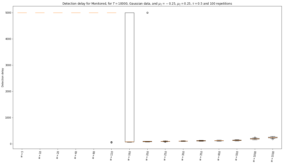
CPU times: user 3.22 s, sys: 877 ms, total: 4.1 s
Wall time: 1min 10s
With a smaller gap, the problem gets harder, and can become impossible to solve (with such a small time horizon).
[379]:
horizon = 10000
firstMean = mu_1 = -0.1
secondMean = mu_2 = 0.1
gap = mu_2 - mu_1
tau = 0.5
[380]:
%%time
_ = view1D_explore_parameters(detection_delay, "Detection delay",
Monitored,
tau=tau,
firstMean=mu_1,
secondMean=mu_2,
horizon=horizon,
repetitions=100,
gaussian=True,
n_jobs=4,
list_of_args_kwargs=list_of_args_kwargs_for_Monitored,
argskwargs2str=argskwargs2str_for_Monitored,
savefig=f"Detection_delay__Monitored__Bernoulli_T1000_N100__{len(list_of_args_kwargs_for_Monitored)}_2",
)
Exploring detection_delay for algorithm <class '__main__.Monitored'>, mu^1 = -0.1, mu^2 = 0.1, and horizon = 10000, tau = 5000...
with 15 values for args, kwargs, and 100 repetitions.
Saving figure with format png, to file 'Detection_delay__Monitored__Bernoulli_T1000_N100__15_2.png'...
Saved! 'Detection_delay__Monitored__Bernoulli_T1000_N100__15_2.png' created of size '25412b', at 'Mon Dec 17 13:16:37 2018' ...
Saving figure with format pdf, to file 'Detection_delay__Monitored__Bernoulli_T1000_N100__15_2.pdf'...
Saved! 'Detection_delay__Monitored__Bernoulli_T1000_N100__15_2.pdf' created of size '16860b', at 'Mon Dec 17 13:16:37 2018' ...
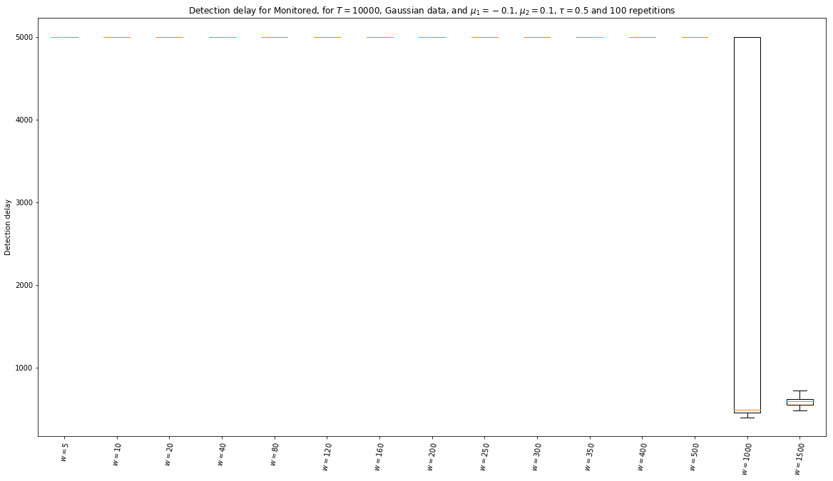
CPU times: user 3.67 s, sys: 735 ms, total: 4.4 s
Wall time: 1min 40s
[381]:
horizon = 10000
firstMean = mu_1 = -0.05
secondMean = mu_2 = 0.05
gap = mu_2 - mu_1
tau = 0.5
[382]:
list_of_args_kwargs_for_Monitored = tuple([
((), {'window_size': w, 'threshold_b': None}) # empty args, kwargs = {window_size=80, threshold_b=None}
for w in [5, 10, 20, 40, 80, 120, 160, 200, 250, 300, 350, 400, 500, 1000, 1500, 2000, 2500, 3000, 4000]
])
[383]:
%%time
_ = view1D_explore_parameters(detection_delay, "Detection delay",
Monitored,
tau=tau,
firstMean=mu_1,
secondMean=mu_2,
horizon=horizon,
repetitions=100,
gaussian=True,
n_jobs=4,
list_of_args_kwargs=list_of_args_kwargs_for_Monitored,
argskwargs2str=argskwargs2str_for_Monitored,
savefig=f"Detection_delay__Monitored__Bernoulli_T1000_N100__{len(list_of_args_kwargs_for_Monitored)}_3",
)
Exploring detection_delay for algorithm <class '__main__.Monitored'>, mu^1 = -0.05, mu^2 = 0.05, and horizon = 10000, tau = 5000...
with 19 values for args, kwargs, and 100 repetitions.
Saving figure with format png, to file 'Detection_delay__Monitored__Bernoulli_T1000_N100__19_3.png'...
Saved! 'Detection_delay__Monitored__Bernoulli_T1000_N100__19_3.png' created of size '28843b', at 'Mon Dec 17 13:19:03 2018' ...
Saving figure with format pdf, to file 'Detection_delay__Monitored__Bernoulli_T1000_N100__19_3.pdf'...
Saved! 'Detection_delay__Monitored__Bernoulli_T1000_N100__19_3.pdf' created of size '17819b', at 'Mon Dec 17 13:19:03 2018' ...
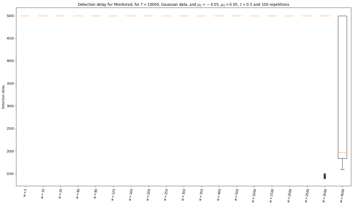
CPU times: user 4.73 s, sys: 1.01 s, total: 5.74 s
Wall time: 2min 26s
Experiments for Bernoulli GLR
[316]:
list_of_args_kwargs_for_BernoulliGLR = tuple([
((), {'mult_threshold_h': h}) # empty args, kwargs = {threshold_h=None}
for h in [0.0001, 0.01, 0.1, 0.5, 0.9, 1, 2, 5, 10, 20, 50, 100, 1000, 10000]
])
[317]:
def argskwargs2str_for_BernoulliGLR(args, kwargs):
h = kwargs['mult_threshold_h']
return fr"$h_0={h:.4g}$" if h is not None else "$h=$'auto'"
Simple Bernoulli problem for BernoulliGLR
First, for a Bernoulli problem:
[319]:
horizon = 1000
firstMean = mu_1 = 0.25
secondMean = mu_2 = 0.75
gap = mu_2 - mu_1
tau = 0.5
[387]:
%%time
_ = view1D_explore_parameters(detection_delay, "Detection delay",
BernoulliGLR,
tau=tau,
firstMean=mu_1,
secondMean=mu_2,
horizon=horizon,
repetitions=10,
gaussian=False,
list_of_args_kwargs=list_of_args_kwargs_for_BernoulliGLR,
argskwargs2str=argskwargs2str_for_BernoulliGLR,
savefig=f"Detection_delay__BernoulliGLR__Bernoulli_T1000_N10__params{len(list_of_args_kwargs_for_BernoulliGLR)}",
)
Exploring detection_delay for algorithm <class '__main__.BernoulliGLR'>, mu^1 = 0.25, mu^2 = 0.75, and horizon = 1000, tau = 500...
with 14 values for args, kwargs, and 10 repetitions.
Saving figure with format png, to file 'Detection_delay__BernoulliGLR__Bernoulli_T1000_N10__params14.png'...
Saved! 'Detection_delay__BernoulliGLR__Bernoulli_T1000_N10__params14.png' created of size '28514b', at 'Mon Dec 17 13:22:02 2018' ...
Saving figure with format pdf, to file 'Detection_delay__BernoulliGLR__Bernoulli_T1000_N10__params14.pdf'...
Saved! 'Detection_delay__BernoulliGLR__Bernoulli_T1000_N10__params14.pdf' created of size '18798b', at 'Mon Dec 17 13:22:02 2018' ...
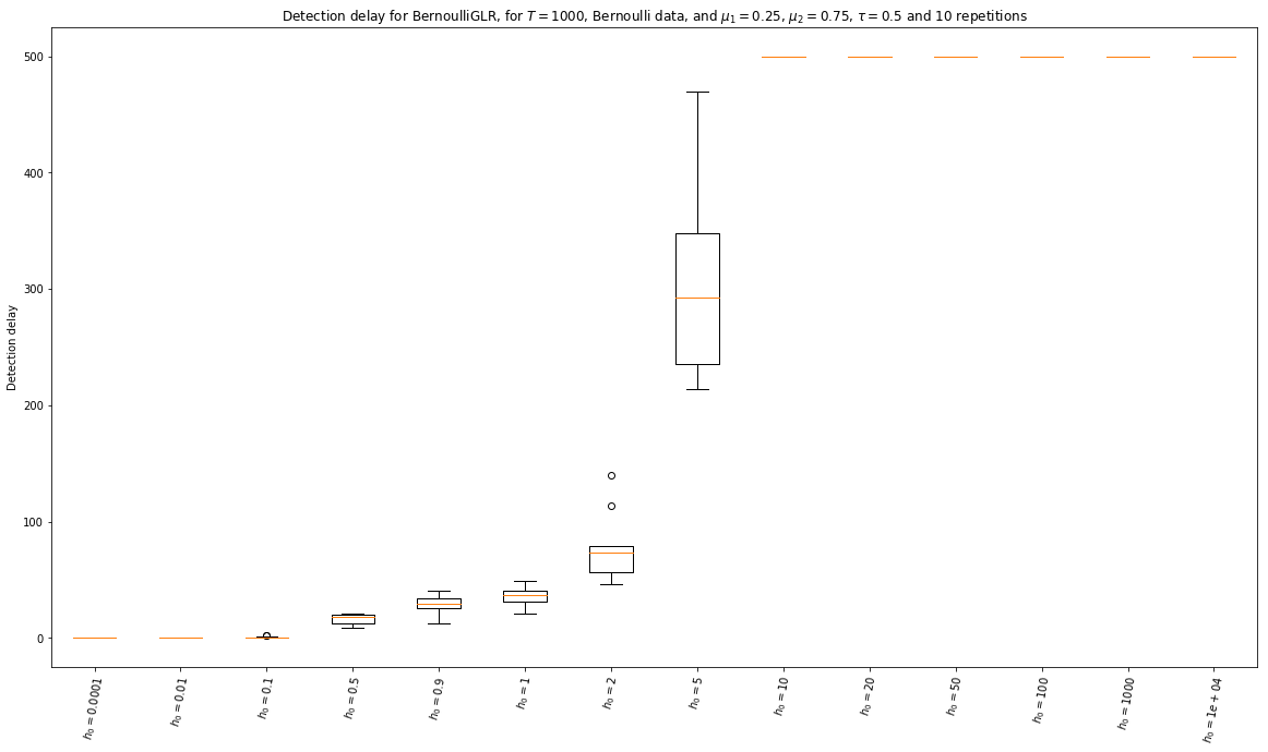
CPU times: user 2.5 s, sys: 728 ms, total: 3.23 s
Wall time: 2min 58s
[388]:
%%time
_ = view1D_explore_parameters(false_alarm, "False alarm probability",
BernoulliGLR,
tau=tau,
firstMean=mu_1,
secondMean=mu_2,
horizon=horizon,
repetitions=10,
gaussian=False,
list_of_args_kwargs=list_of_args_kwargs_for_BernoulliGLR,
argskwargs2str=argskwargs2str_for_BernoulliGLR,
savefig=f"False_alarm__BernoulliGLR__Bernoulli_T1000_N10__params{len(list_of_args_kwargs_for_BernoulliGLR)}",
)
Exploring false_alarm for algorithm <class '__main__.BernoulliGLR'>, mu^1 = 0.25, mu^2 = 0.75, and horizon = 1000, tau = 500...
with 14 values for args, kwargs, and 20 repetitions.
Saving figure with format png, to file 'False_alarm__BernoulliGLR__Bernoulli_T1000_N20__params14.png'...
Saved! 'False_alarm__BernoulliGLR__Bernoulli_T1000_N20__params14.png' created of size '27744b', at 'Mon Dec 17 13:25:04 2018' ...
Saving figure with format pdf, to file 'False_alarm__BernoulliGLR__Bernoulli_T1000_N20__params14.pdf'...
Saved! 'False_alarm__BernoulliGLR__Bernoulli_T1000_N20__params14.pdf' created of size '18967b', at 'Mon Dec 17 13:25:05 2018' ...

CPU times: user 2.02 s, sys: 750 ms, total: 2.77 s
Wall time: 3min 2s
[389]:
%%time
_ = view1D_explore_parameters(missed_detection, "Missed detection probability",
BernoulliGLR,
tau=tau,
firstMean=mu_1,
secondMean=mu_2,
horizon=horizon,
repetitions=10,
gaussian=False,
list_of_args_kwargs=list_of_args_kwargs_for_BernoulliGLR,
argskwargs2str=argskwargs2str_for_BernoulliGLR,
savefig=f"Missed_detection__BernoulliGLR__Bernoulli_T1000_N10__params{len(list_of_args_kwargs_for_BernoulliGLR)}",
)
Exploring missed_detection for algorithm <class '__main__.BernoulliGLR'>, mu^1 = 0.25, mu^2 = 0.75, and horizon = 1000, tau = 500...
with 14 values for args, kwargs, and 20 repetitions.
Saving figure with format png, to file 'Missed_detection__BernoulliGLR__Bernoulli_T1000_N100__params14.png'...
Saved! 'Missed_detection__BernoulliGLR__Bernoulli_T1000_N100__params14.png' created of size '28800b', at 'Mon Dec 17 13:30:58 2018' ...
Saving figure with format pdf, to file 'Missed_detection__BernoulliGLR__Bernoulli_T1000_N100__params14.pdf'...
Saved! 'Missed_detection__BernoulliGLR__Bernoulli_T1000_N100__params14.pdf' created of size '18821b', at 'Mon Dec 17 13:30:58 2018' ...
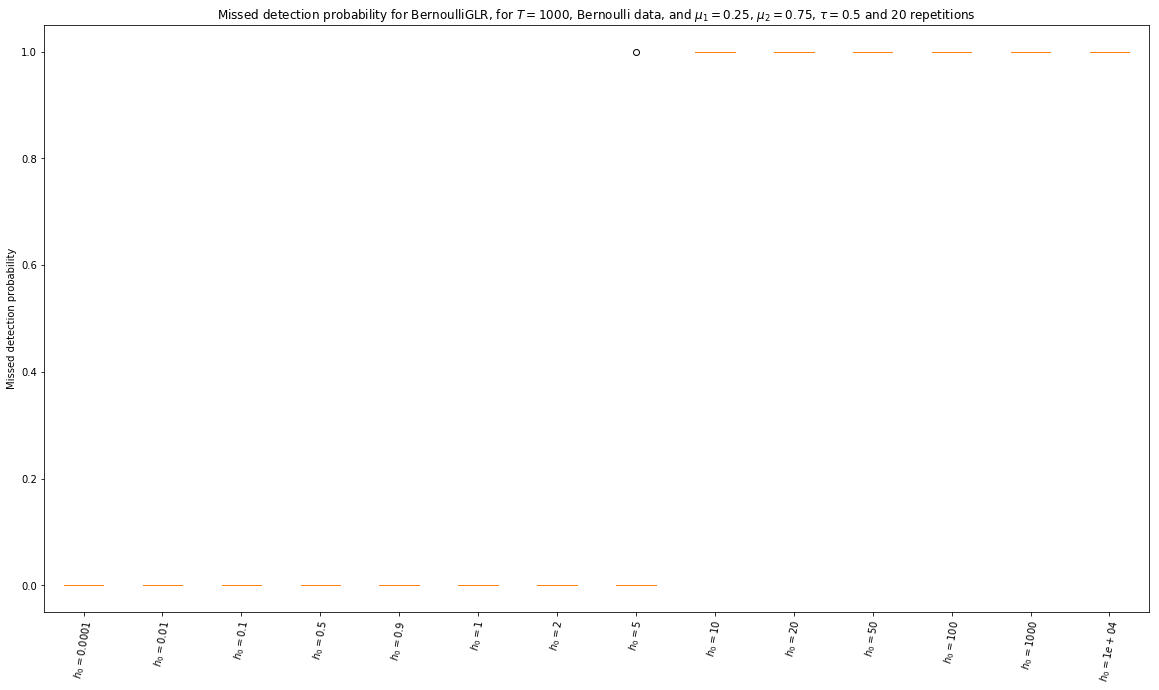
CPU times: user 2.07 s, sys: 722 ms, total: 2.79 s
Wall time: 5min 53s
Medium Bernoulli problem for BernoulliGLR
Then, for a harder Bernoulli problem. Here the gap is \(\frac{1}{\sqrt{2}}\) smaller, \(\Delta=\frac{1}{2\sqrt{2}}\), so the complexity of the problem should be twice as hard (it scales as \(\propto \frac{1}{\Delta^2}\)).
[329]:
horizon = 1000
firstMean = mu_1 = 0.25
gap = 1/2 / np.sqrt(2)
print(f"Gap = {gap}")
secondMean = mu_2 = mu_1 + gap
tau = 0.5
Gap = 0.35355339059327373
[330]:
%%time
_ = view1D_explore_parameters(detection_delay, "Detection delay",
BernoulliGLR,
tau=tau,
firstMean=mu_1,
secondMean=mu_2,
horizon=horizon,
repetitions=10,
gaussian=False,
list_of_args_kwargs=list_of_args_kwargs_for_BernoulliGLR,
argskwargs2str=argskwargs2str_for_BernoulliGLR,
savefig=f"Detection_delay__BernoulliGLR__Bernoulli_T1000_N10__params{len(list_of_args_kwargs_for_BernoulliGLR)}_2",
)
Exploring detection_delay for algorithm <class '__main__.BernoulliGLR'>, mu^1 = 0.25, mu^2 = 0.6035533905932737, and horizon = 1000, tau = 500...
with 14 values for args, kwargs, and 10 repetitions.
Saving figure with format png, to file 'Detection_delay__BernoulliGLR__Bernoulli_T1000_N10__params14_2.png'...
Saved! 'Detection_delay__BernoulliGLR__Bernoulli_T1000_N10__params14_2.png' created of size '28283b', at 'Tue Dec 18 14:09:53 2018' ...
Saving figure with format pdf, to file 'Detection_delay__BernoulliGLR__Bernoulli_T1000_N10__params14_2.pdf'...
Saved! 'Detection_delay__BernoulliGLR__Bernoulli_T1000_N10__params14_2.pdf' created of size '18667b', at 'Tue Dec 18 14:09:53 2018' ...
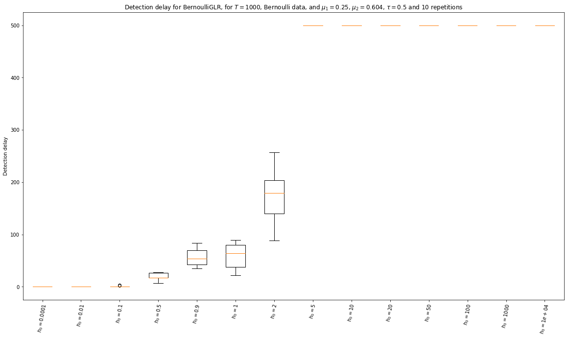
CPU times: user 2.5 s, sys: 1.03 s, total: 3.53 s
Wall time: 2min 1s
[331]:
%%time
_ = view1D_explore_parameters(false_alarm, "False alarm probability",
BernoulliGLR,
tau=tau,
firstMean=mu_1,
secondMean=mu_2,
horizon=horizon,
repetitions=10,
gaussian=False,
list_of_args_kwargs=list_of_args_kwargs_for_BernoulliGLR,
argskwargs2str=argskwargs2str_for_BernoulliGLR,
savefig=f"False_alarm__BernoulliGLR__Bernoulli_T1000_N10__params{len(list_of_args_kwargs_for_BernoulliGLR)}_2",
)
Exploring false_alarm for algorithm <class '__main__.BernoulliGLR'>, mu^1 = 0.25, mu^2 = 0.6035533905932737, and horizon = 1000, tau = 500...
with 14 values for args, kwargs, and 10 repetitions.
Saving figure with format png, to file 'False_alarm__BernoulliGLR__Bernoulli_T1000_N10__params14_2.png'...
Saved! 'False_alarm__BernoulliGLR__Bernoulli_T1000_N10__params14_2.png' created of size '27700b', at 'Tue Dec 18 14:10:51 2018' ...
Saving figure with format pdf, to file 'False_alarm__BernoulliGLR__Bernoulli_T1000_N10__params14_2.pdf'...
Saved! 'False_alarm__BernoulliGLR__Bernoulli_T1000_N10__params14_2.pdf' created of size '18420b', at 'Tue Dec 18 14:10:52 2018' ...
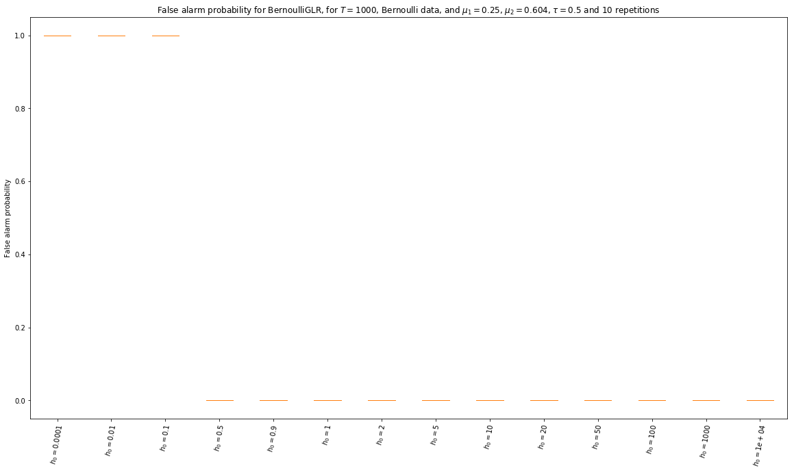
CPU times: user 2.58 s, sys: 554 ms, total: 3.13 s
Wall time: 58.3 s
[332]:
%%time
_ = view1D_explore_parameters(missed_detection, "Missed detection probability",
BernoulliGLR,
tau=tau,
firstMean=mu_1,
secondMean=mu_2,
horizon=horizon,
repetitions=10,
gaussian=False,
list_of_args_kwargs=list_of_args_kwargs_for_BernoulliGLR,
argskwargs2str=argskwargs2str_for_BernoulliGLR,
savefig=f"Missed_detection__BernoulliGLR__Bernoulli_T1000_N10__params{len(list_of_args_kwargs_for_BernoulliGLR)}_2",
)
Exploring missed_detection for algorithm <class '__main__.BernoulliGLR'>, mu^1 = 0.25, mu^2 = 0.6035533905932737, and horizon = 1000, tau = 500...
with 14 values for args, kwargs, and 10 repetitions.
Saving figure with format png, to file 'Missed_detection__BernoulliGLR__Bernoulli_T1000_N10__params14_2.png'...
Saved! 'Missed_detection__BernoulliGLR__Bernoulli_T1000_N10__params14_2.png' created of size '28833b', at 'Tue Dec 18 14:13:00 2018' ...
Saving figure with format pdf, to file 'Missed_detection__BernoulliGLR__Bernoulli_T1000_N10__params14_2.pdf'...
Saved! 'Missed_detection__BernoulliGLR__Bernoulli_T1000_N10__params14_2.pdf' created of size '18424b', at 'Tue Dec 18 14:13:01 2018' ...
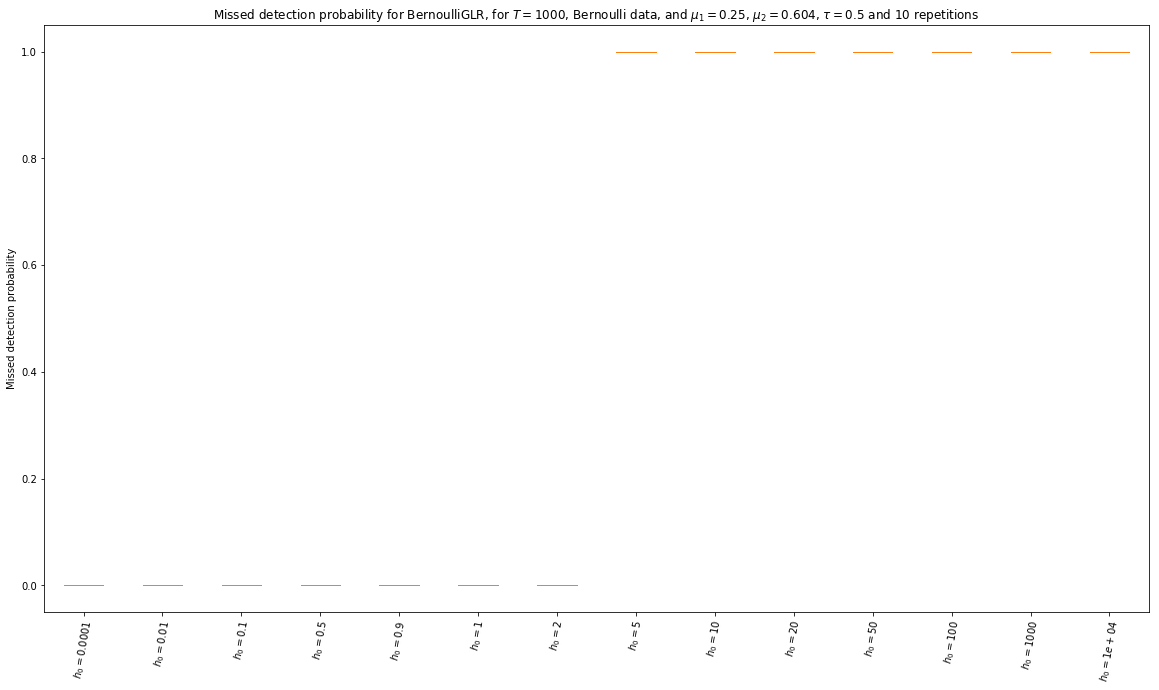
CPU times: user 2.61 s, sys: 606 ms, total: 3.22 s
Wall time: 2min 8s
Harder Bernoulli problem for BernoulliGLR
Then, for a really harder Bernoulli problem. Here the gap is again smaller, \(\Delta=\frac{1}{10}\), so the complexity of the problem should (again) much harder (it scales as \(\propto \frac{1}{\Delta^2}\)).
[359]:
list_of_args_kwargs_for_BernoulliGLR = tuple([
((), {'mult_threshold_h': h}) # empty args, kwargs = {threshold_h=None}
for h in [0.05, 0.1, 0.2, 0.3, 0.4, 0.5, 0.6, 0.7, 0.8, 0.9, 1, 2]
])
[360]:
horizon = 1000
firstMean = mu_1 = 0.25
gap = 0.1
print(f"Gap = {gap}")
secondMean = mu_2 = mu_1 + gap
tau = 0.5
Gap = 0.1
[361]:
%%time
_ = view1D_explore_parameters(detection_delay, "Detection delay",
BernoulliGLR,
tau=tau,
firstMean=mu_1,
secondMean=mu_2,
horizon=horizon,
repetitions=100,
gaussian=False,
list_of_args_kwargs=list_of_args_kwargs_for_BernoulliGLR,
argskwargs2str=argskwargs2str_for_BernoulliGLR,
savefig=f"Detection_delay__BernoulliGLR__Bernoulli_T1000_N100__params{len(list_of_args_kwargs_for_BernoulliGLR)}_4",
)
Exploring detection_delay for algorithm <class '__main__.BernoulliGLR'>, mu^1 = 0.25, mu^2 = 0.35, and horizon = 1000, tau = 500...
with 12 values for args, kwargs, and 100 repetitions.
Saving figure with format png, to file 'Detection_delay__BernoulliGLR__Bernoulli_T1000_N100__params12_4.png'...
Saved! 'Detection_delay__BernoulliGLR__Bernoulli_T1000_N100__params12_4.png' created of size '28649b', at 'Tue Dec 18 15:29:35 2018' ...
Saving figure with format pdf, to file 'Detection_delay__BernoulliGLR__Bernoulli_T1000_N100__params12_4.pdf'...
Saved! 'Detection_delay__BernoulliGLR__Bernoulli_T1000_N100__params12_4.pdf' created of size '20352b', at 'Tue Dec 18 15:29:35 2018' ...
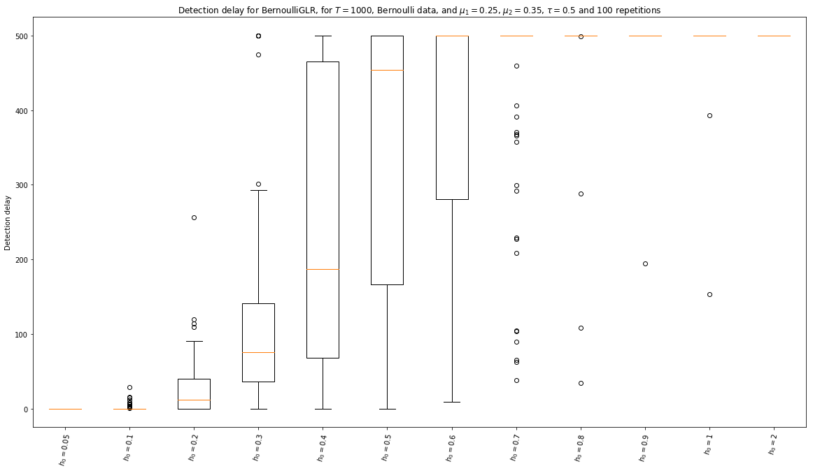
CPU times: user 2.74 s, sys: 768 ms, total: 3.51 s
Wall time: 18min 11s
[362]:
%%time
_ = view1D_explore_parameters(false_alarm, "False alarm probability",
BernoulliGLR,
tau=tau,
firstMean=mu_1,
secondMean=mu_2,
horizon=horizon,
repetitions=100,
gaussian=False,
list_of_args_kwargs=list_of_args_kwargs_for_BernoulliGLR,
argskwargs2str=argskwargs2str_for_BernoulliGLR,
savefig=f"False_alarm__BernoulliGLR__Bernoulli_T1000_N100__params{len(list_of_args_kwargs_for_BernoulliGLR)}_5",
)
Exploring false_alarm for algorithm <class '__main__.BernoulliGLR'>, mu^1 = 0.25, mu^2 = 0.35, and horizon = 1000, tau = 500...
with 12 values for args, kwargs, and 100 repetitions.
Saving figure with format png, to file 'False_alarm__BernoulliGLR__Bernoulli_T1000_N100__params12_5.png'...
Saved! 'False_alarm__BernoulliGLR__Bernoulli_T1000_N100__params12_5.png' created of size '23546b', at 'Tue Dec 18 15:36:09 2018' ...
Saving figure with format pdf, to file 'False_alarm__BernoulliGLR__Bernoulli_T1000_N100__params12_5.pdf'...
Saved! 'False_alarm__BernoulliGLR__Bernoulli_T1000_N100__params12_5.pdf' created of size '19260b', at 'Tue Dec 18 15:36:09 2018' ...
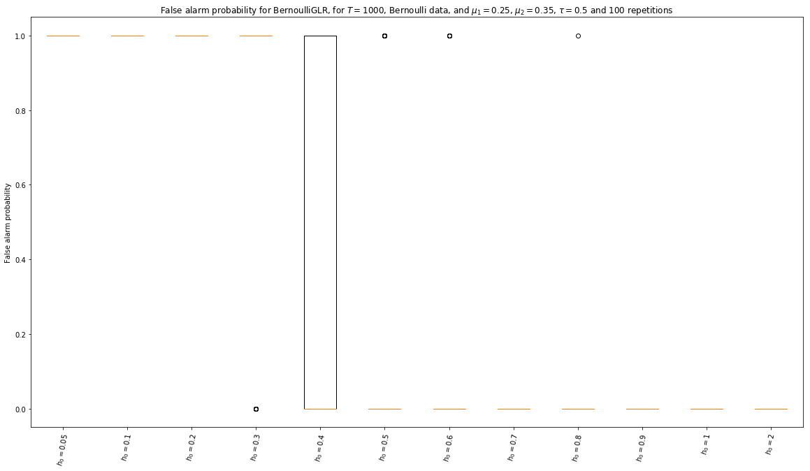
CPU times: user 2.23 s, sys: 795 ms, total: 3.03 s
Wall time: 6min 34s
[363]:
%%time
_ = view1D_explore_parameters(missed_detection, "Missed detection probability",
BernoulliGLR,
tau=tau,
firstMean=mu_1,
secondMean=mu_2,
horizon=horizon,
repetitions=100,
gaussian=False,
list_of_args_kwargs=list_of_args_kwargs_for_BernoulliGLR,
argskwargs2str=argskwargs2str_for_BernoulliGLR,
savefig=f"Missed_detection__BernoulliGLR__Bernoulli_T1000_N100__params{len(list_of_args_kwargs_for_BernoulliGLR)}_5",
)
Exploring missed_detection for algorithm <class '__main__.BernoulliGLR'>, mu^1 = 0.25, mu^2 = 0.35, and horizon = 1000, tau = 500...
with 12 values for args, kwargs, and 100 repetitions.
Saving figure with format png, to file 'Missed_detection__BernoulliGLR__Bernoulli_T1000_N100__params12_5.png'...
Saved! 'Missed_detection__BernoulliGLR__Bernoulli_T1000_N100__params12_5.png' created of size '24903b', at 'Tue Dec 18 15:56:37 2018' ...
Saving figure with format pdf, to file 'Missed_detection__BernoulliGLR__Bernoulli_T1000_N100__params12_5.pdf'...
Saved! 'Missed_detection__BernoulliGLR__Bernoulli_T1000_N100__params12_5.pdf' created of size '19895b', at 'Tue Dec 18 15:56:37 2018' ...
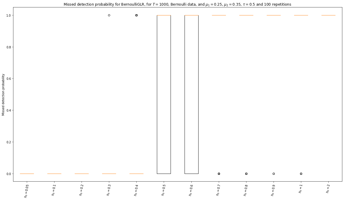
CPU times: user 3.43 s, sys: 463 ms, total: 3.89 s
Wall time: 20min 28s
Easy Gaussian problem for BernoulliGLR
And now on Gaussian problems:
[266]:
horizon = 1000
firstMean = mu_1 = -0.25
secondMean = mu_2 = 0.25
gap = mu_2 - mu_1
tau = 0.5
[267]:
%%time
_ = view1D_explore_parameters(detection_delay, "Detection delay",
BernoulliGLR,
tau=tau,
firstMean=mu_1,
secondMean=mu_2,
horizon=horizon,
repetitions=10,
gaussian=True,
list_of_args_kwargs=list_of_args_kwargs_for_BernoulliGLR,
argskwargs2str=argskwargs2str_for_BernoulliGLR,
savefig=f"Detection_delay__BernoulliGLR__Gaussian_T1000_N10__params{len(list_of_args_kwargs_for_BernoulliGLR)}",
)
Exploring detection_delay for algorithm <class '__main__.BernoulliGLR'>, mu^1 = -0.25, mu^2 = 0.25, and horizon = 1000, tau = 500...
with 14 values for args, kwargs, and 10 repetitions.
Saving figure with format png, to file 'Detection_delay__BernoulliGLR__Gaussian_T1000_N10__params14.png'...
Saved! 'Detection_delay__BernoulliGLR__Gaussian_T1000_N10__params14.png' created of size '29505b', at 'Mon Dec 17 19:15:23 2018' ...
Saving figure with format pdf, to file 'Detection_delay__BernoulliGLR__Gaussian_T1000_N10__params14.pdf'...
Saved! 'Detection_delay__BernoulliGLR__Gaussian_T1000_N10__params14.pdf' created of size '19719b', at 'Mon Dec 17 19:15:23 2018' ...
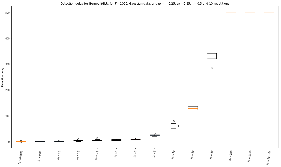
CPU times: user 2.37 s, sys: 777 ms, total: 3.15 s
Wall time: 54.6 s
[270]:
%%time
_ = view1D_explore_parameters(false_alarm, "False alarm probability",
BernoulliGLR,
tau=tau,
firstMean=mu_1,
secondMean=mu_2,
horizon=horizon,
repetitions=50,
gaussian=True,
list_of_args_kwargs=list_of_args_kwargs_for_BernoulliGLR,
argskwargs2str=argskwargs2str_for_BernoulliGLR,
savefig=f"False_alarm__BernoulliGLR__Gaussian_T1000_N10__params{len(list_of_args_kwargs_for_BernoulliGLR)}",
)
Exploring false_alarm for algorithm <class '__main__.BernoulliGLR'>, mu^1 = -0.25, mu^2 = 0.25, and horizon = 1000, tau = 500...
with 14 values for args, kwargs, and 50 repetitions.
Saving figure with format png, to file 'False_alarm__BernoulliGLR__Gaussian_T1000_N10__params14.png'...
Saved! 'False_alarm__BernoulliGLR__Gaussian_T1000_N10__params14.png' created of size '27885b', at 'Mon Dec 17 19:17:55 2018' ...
Saving figure with format pdf, to file 'False_alarm__BernoulliGLR__Gaussian_T1000_N10__params14.pdf'...
Saved! 'False_alarm__BernoulliGLR__Gaussian_T1000_N10__params14.pdf' created of size '19225b', at 'Mon Dec 17 19:17:55 2018' ...
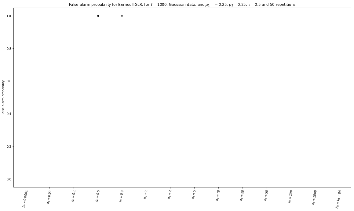
CPU times: user 2.06 s, sys: 745 ms, total: 2.8 s
Wall time: 2min 54s
[392]:
horizon = 1000
firstMean = mu_1 = -0.05
secondMean = mu_2 = 0.05
gap = mu_2 - mu_1
tau = 0.5
[393]:
%%time
_ = view1D_explore_parameters(detection_delay, "Detection delay",
BernoulliGLR,
tau=tau,
firstMean=mu_1,
secondMean=mu_2,
horizon=horizon,
repetitions=10,
gaussian=True,
list_of_args_kwargs=list_of_args_kwargs_for_BernoulliGLR,
argskwargs2str=argskwargs2str_for_BernoulliGLR,
savefig=f"Detection_delay__BernoulliGLR__Gaussian_T1000_N10__params{len(list_of_args_kwargs_for_BernoulliGLR)}_2",
)
Exploring detection_delay for algorithm <class '__main__.BernoulliGLR'>, mu^1 = -0.05, mu^2 = 0.05, and horizon = 1000, tau = 500...
with 14 values for args, kwargs, and 10 repetitions.
Saving figure with format png, to file 'Detection_delay__BernoulliGLR__Gaussian_T1000_N10__params14_2.png'...
Saved! 'Detection_delay__BernoulliGLR__Gaussian_T1000_N10__params14_2.png' created of size '28975b', at 'Mon Dec 17 13:33:14 2018' ...
Saving figure with format pdf, to file 'Detection_delay__BernoulliGLR__Gaussian_T1000_N10__params14_2.pdf'...
Saved! 'Detection_delay__BernoulliGLR__Gaussian_T1000_N10__params14_2.pdf' created of size '19241b', at 'Mon Dec 17 13:33:14 2018' ...
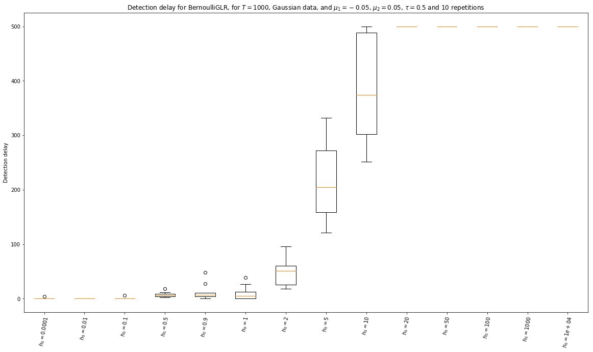
CPU times: user 2.02 s, sys: 767 ms, total: 2.79 s
Wall time: 2min 15s
[394]:
%%time
_ = view1D_explore_parameters(false_alarm, "False alarm probability",
BernoulliGLR,
tau=tau,
firstMean=mu_1,
secondMean=mu_2,
horizon=horizon,
repetitions=10,
gaussian=True,
list_of_args_kwargs=list_of_args_kwargs_for_BernoulliGLR,
argskwargs2str=argskwargs2str_for_BernoulliGLR,
savefig=f"False_alarm__BernoulliGLR__Gaussian_T1000_N10__params{len(list_of_args_kwargs_for_BernoulliGLR)}_2",
)
Exploring false_alarm for algorithm <class '__main__.BernoulliGLR'>, mu^1 = -0.05, mu^2 = 0.05, and horizon = 1000, tau = 500...
with 14 values for args, kwargs, and 10 repetitions.
Saving figure with format png, to file 'False_alarm__BernoulliGLR__Gaussian_T1000_N10__params14_2.png'...
Saved! 'False_alarm__BernoulliGLR__Gaussian_T1000_N10__params14_2.png' created of size '27567b', at 'Mon Dec 17 13:34:09 2018' ...
Saving figure with format pdf, to file 'False_alarm__BernoulliGLR__Gaussian_T1000_N10__params14_2.pdf'...
Saved! 'False_alarm__BernoulliGLR__Gaussian_T1000_N10__params14_2.pdf' created of size '18886b', at 'Mon Dec 17 13:34:10 2018' ...
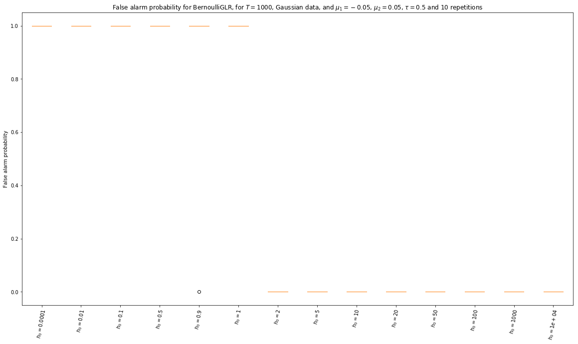
CPU times: user 2.03 s, sys: 682 ms, total: 2.71 s
Wall time: 55.5 s
[271]:
%%time
_ = view1D_explore_parameters(missed_detection, "Missed detection probability",
BernoulliGLR,
tau=tau,
firstMean=mu_1,
secondMean=mu_2,
horizon=horizon,
repetitions=10,
gaussian=True,
list_of_args_kwargs=list_of_args_kwargs_for_BernoulliGLR,
argskwargs2str=argskwargs2str_for_BernoulliGLR,
savefig=f"Missed_detection__BernoulliGLR__Gaussian_T1000_N10__params{len(list_of_args_kwargs_for_BernoulliGLR)}_2",
)
Exploring missed_detection for algorithm <class '__main__.BernoulliGLR'>, mu^1 = -0.25, mu^2 = 0.25, and horizon = 1000, tau = 500...
with 14 values for args, kwargs, and 10 repetitions.
Saving figure with format png, to file 'Missed_detection__BernoulliGLR__Gaussian_T1000_N10__params14_2.png'...
Saved! 'Missed_detection__BernoulliGLR__Gaussian_T1000_N10__params14_2.png' created of size '28537b', at 'Mon Dec 17 19:22:44 2018' ...
Saving figure with format pdf, to file 'Missed_detection__BernoulliGLR__Gaussian_T1000_N10__params14_2.pdf'...
Saved! 'Missed_detection__BernoulliGLR__Gaussian_T1000_N10__params14_2.pdf' created of size '18662b', at 'Mon Dec 17 19:22:44 2018' ...
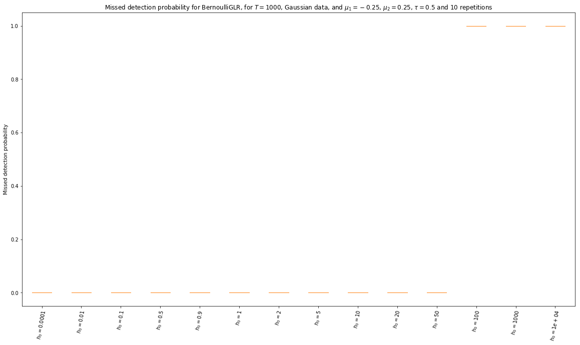
CPU times: user 2.61 s, sys: 573 ms, total: 3.18 s
Wall time: 58.3 s
Experiments for Gaussian GLR
[272]:
list_of_args_kwargs_for_GaussianGLR = tuple([
((), {'mult_threshold_h': h}) # empty args, kwargs = {threshold_h=None}
for h in [0.0001, 0.01, 0.1, 0.5, 0.9, 1, 2, 5, 10, 20, 50, 100, 1000, 10000]
])
[273]:
def argskwargs2str_for_GaussianGLR(args, kwargs):
h = kwargs['mult_threshold_h']
return fr"$h={h:.4g}$" if h is not None else "$h=$'auto'"
First, for a Bernoulli problem:
[274]:
horizon = 1000
firstMean = mu_1 = 0.25
secondMean = mu_2 = 0.75
gap = mu_2 - mu_1
tau = 0.5
[275]:
%%time
_ = view1D_explore_parameters(detection_delay, "Detection delay",
GaussianGLR,
tau=tau,
firstMean=mu_1,
secondMean=mu_2,
horizon=horizon,
repetitions=10,
gaussian=False,
list_of_args_kwargs=list_of_args_kwargs_for_GaussianGLR,
argskwargs2str=argskwargs2str_for_GaussianGLR,
savefig=f"Detection_delay__GaussianGLR__Bernoulli_T1000_N10__params{len(list_of_args_kwargs_for_GaussianGLR)}_2",
)
Exploring detection_delay for algorithm <class '__main__.GaussianGLR'>, mu^1 = 0.25, mu^2 = 0.75, and horizon = 1000, tau = 500...
with 14 values for args, kwargs, and 10 repetitions.
Saving figure with format png, to file 'Detection_delay__GaussianGLR__Bernoulli_T1000_N10__params14_2.png'...
Saved! 'Detection_delay__GaussianGLR__Bernoulli_T1000_N10__params14_2.png' created of size '27449b', at 'Mon Dec 17 19:24:19 2018' ...
Saving figure with format pdf, to file 'Detection_delay__GaussianGLR__Bernoulli_T1000_N10__params14_2.pdf'...
Saved! 'Detection_delay__GaussianGLR__Bernoulli_T1000_N10__params14_2.pdf' created of size '18488b', at 'Mon Dec 17 19:24:20 2018' ...
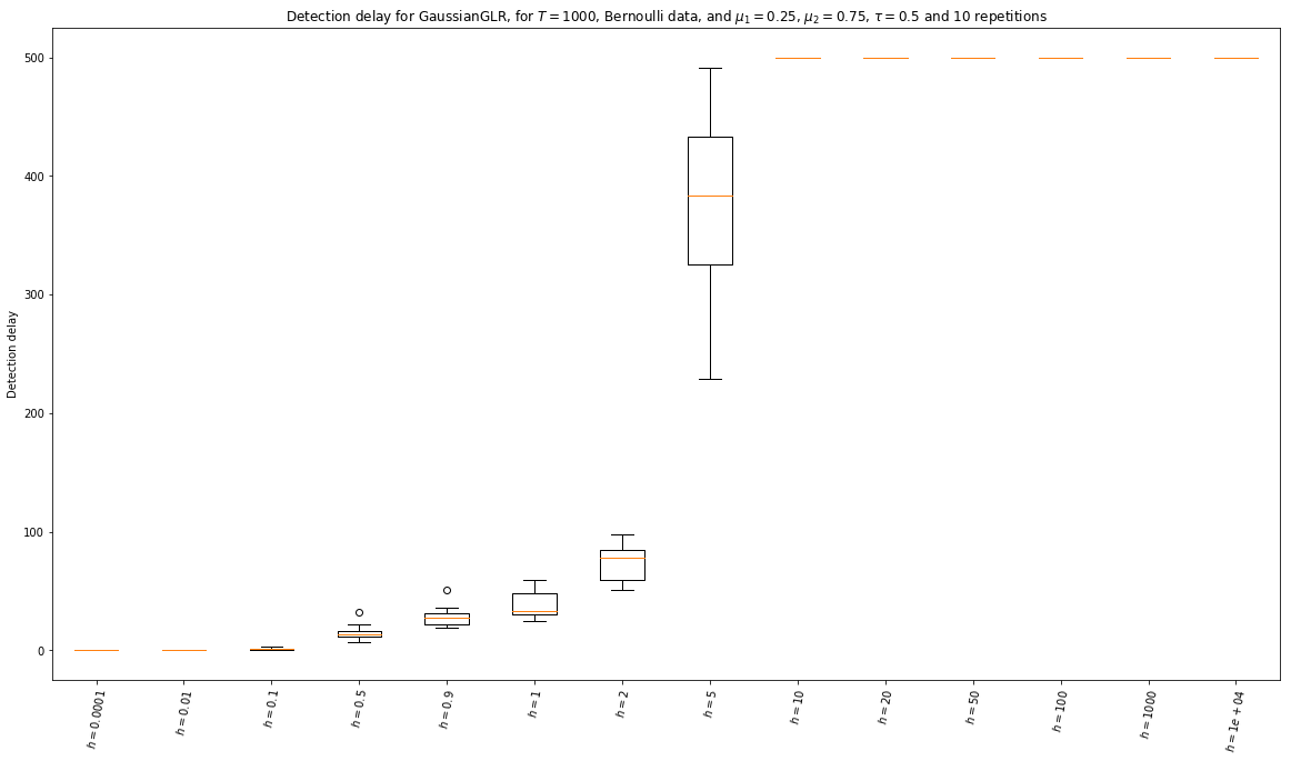
CPU times: user 2.17 s, sys: 685 ms, total: 2.85 s
Wall time: 1min 2s
[276]:
%%time
_ = view1D_explore_parameters(false_alarm, "False alarm",
GaussianGLR,
tau=tau,
firstMean=mu_1,
secondMean=mu_2,
horizon=horizon,
repetitions=10,
gaussian=False,
list_of_args_kwargs=list_of_args_kwargs_for_GaussianGLR,
argskwargs2str=argskwargs2str_for_GaussianGLR,
savefig=f"False_alarm__GaussianGLR__Bernoulli_T1000_N10__params{len(list_of_args_kwargs_for_GaussianGLR)}_2",
)
Exploring false_alarm for algorithm <class '__main__.GaussianGLR'>, mu^1 = 0.25, mu^2 = 0.75, and horizon = 1000, tau = 500...
with 14 values for args, kwargs, and 10 repetitions.
Saving figure with format png, to file 'False_alarm__GaussianGLR__Bernoulli_T1000_N10__params14_2.png'...
Saved! 'False_alarm__GaussianGLR__Bernoulli_T1000_N10__params14_2.png' created of size '24897b', at 'Mon Dec 17 19:25:38 2018' ...
Saving figure with format pdf, to file 'False_alarm__GaussianGLR__Bernoulli_T1000_N10__params14_2.pdf'...
Saved! 'False_alarm__GaussianGLR__Bernoulli_T1000_N10__params14_2.pdf' created of size '18321b', at 'Mon Dec 17 19:25:39 2018' ...
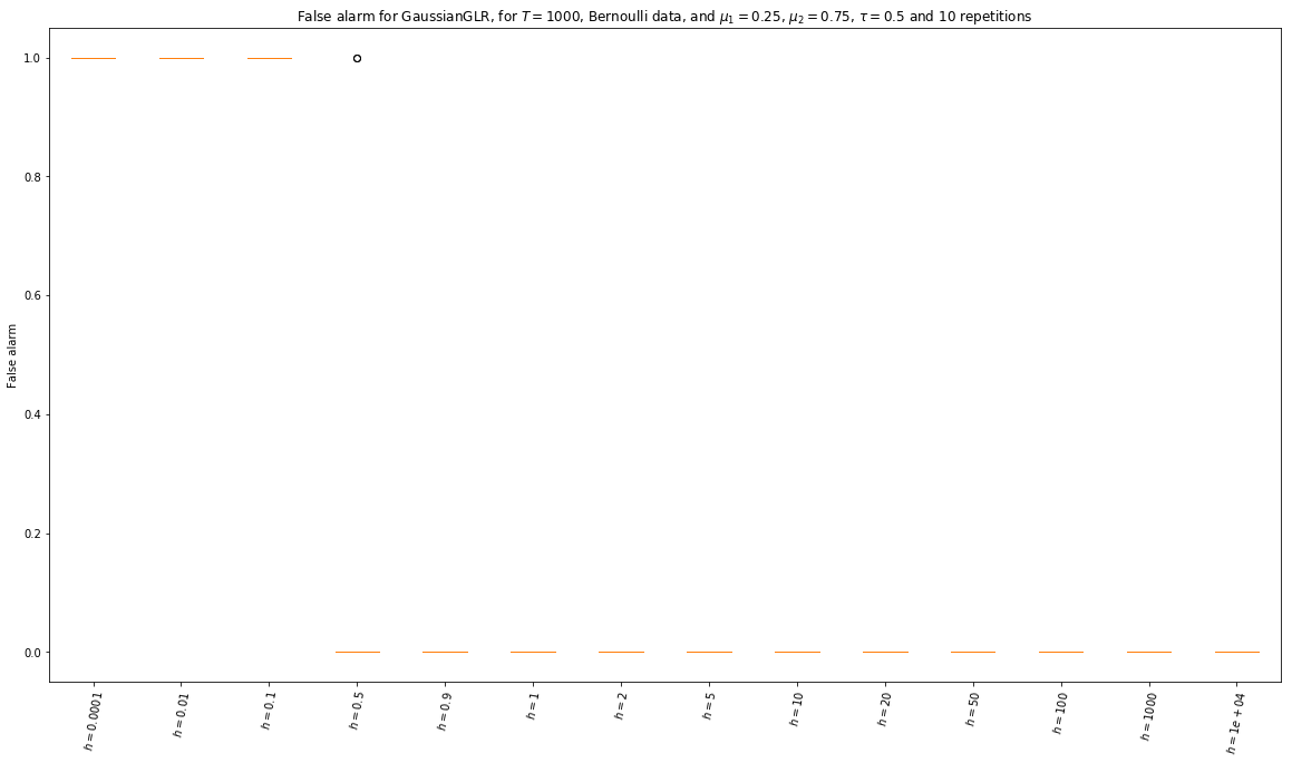
CPU times: user 2.47 s, sys: 609 ms, total: 3.08 s
Wall time: 42.4 s
Then, for a Gaussian problem:
[277]:
horizon = 1000
firstMean = mu_1 = -0.1
secondMean = mu_2 = 0.1
gap = mu_2 - mu_1
tau = 0.5
[278]:
%%time
_ = view1D_explore_parameters(detection_delay, "Detection delay",
GaussianGLR,
tau=tau,
firstMean=mu_1,
secondMean=mu_2,
horizon=horizon,
repetitions=10,
gaussian=True,
list_of_args_kwargs=list_of_args_kwargs_for_GaussianGLR,
argskwargs2str=argskwargs2str_for_GaussianGLR,
savefig=f"Detection_delay__GaussianGLR__Gaussian_T1000_N10__params{len(list_of_args_kwargs_for_GaussianGLR)}_2",
)
Exploring detection_delay for algorithm <class '__main__.GaussianGLR'>, mu^1 = -0.1, mu^2 = 0.1, and horizon = 1000, tau = 500...
with 14 values for args, kwargs, and 10 repetitions.
Saving figure with format png, to file 'Detection_delay__GaussianGLR__Gaussian_T1000_N10__params14_2.png'...
Saved! 'Detection_delay__GaussianGLR__Gaussian_T1000_N10__params14_2.png' created of size '26437b', at 'Mon Dec 17 19:27:43 2018' ...
Saving figure with format pdf, to file 'Detection_delay__GaussianGLR__Gaussian_T1000_N10__params14_2.pdf'...
Saved! 'Detection_delay__GaussianGLR__Gaussian_T1000_N10__params14_2.pdf' created of size '17669b', at 'Mon Dec 17 19:27:43 2018' ...
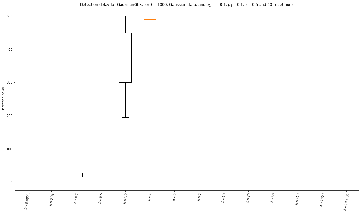
CPU times: user 2.58 s, sys: 641 ms, total: 3.22 s
Wall time: 1min 53s
And for a harder Gaussian problem:
[279]:
horizon = 1000
firstMean = mu_1 = -0.01
secondMean = mu_2 = 0.01
gap = mu_2 - mu_1
tau = 0.5
[280]:
%%time
_ = view1D_explore_parameters(detection_delay, "Detection delay",
GaussianGLR,
tau=tau,
firstMean=mu_1,
secondMean=mu_2,
horizon=horizon,
repetitions=10,
gaussian=True,
list_of_args_kwargs=list_of_args_kwargs_for_GaussianGLR,
argskwargs2str=argskwargs2str_for_GaussianGLR,
savefig=f"Detection_delay__GaussianGLR__Gaussian_T1000_N10__params{len(list_of_args_kwargs_for_GaussianGLR)}_3",
)
Exploring detection_delay for algorithm <class '__main__.GaussianGLR'>, mu^1 = -0.01, mu^2 = 0.01, and horizon = 1000, tau = 500...
with 14 values for args, kwargs, and 10 repetitions.
Saving figure with format png, to file 'Detection_delay__GaussianGLR__Gaussian_T1000_N10__params14_3.png'...
Saved! 'Detection_delay__GaussianGLR__Gaussian_T1000_N10__params14_3.png' created of size '26079b', at 'Mon Dec 17 19:29:35 2018' ...
Saving figure with format pdf, to file 'Detection_delay__GaussianGLR__Gaussian_T1000_N10__params14_3.pdf'...
Saved! 'Detection_delay__GaussianGLR__Gaussian_T1000_N10__params14_3.pdf' created of size '17507b', at 'Mon Dec 17 19:29:36 2018' ...
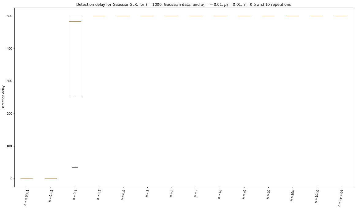
CPU times: user 2.63 s, sys: 425 ms, total: 3.05 s
Wall time: 1min 52s
Experiments for CUSUM
[282]:
list_of_args_kwargs_for_CUSUM = tuple([
((), {'epsilon': epsilon, 'threshold_h': h, 'M': M}) # empty args, kwargs = {epsilon=0.5, threshold_h=None, M=100}
for epsilon in [0.05, 0.1, 0.5, 0.75, 0.9]
for h in [None, 0.01, 0.1, 1, 10]
for M in [50, 100, 150, 200, 500]
])
[283]:
print(f"Exploring {len(list_of_args_kwargs_for_CUSUM)} different values of (h, epsilon, M) for CUSUM...")
Exploring 125 different values of (h, epsilon, M) for CUSUM...
[284]:
def argskwargs2str_for_CUSUM(args, kwargs):
epsilon = kwargs['epsilon']
M = kwargs['M']
h = kwargs['threshold_h']
return fr"$\varepsilon={epsilon:.4g}$, $M={M}$, $h={h:.4g}$" if h is not None else fr"$\varepsilon={epsilon:.4g}$, $M={M}$, $h=$'auto'"
First, for a Bernoulli problem:
[305]:
horizon = 1000
firstMean = mu_1 = 0.25
secondMean = mu_2 = 0.75
gap = mu_2 - mu_1
tau = 0.5
[408]:
%%time
_ = view1D_explore_parameters(detection_delay, "Detection delay",
CUSUM,
tau=tau,
firstMean=mu_1,
secondMean=mu_2,
horizon=horizon,
repetitions=10,
gaussian=False,
list_of_args_kwargs=list_of_args_kwargs_for_CUSUM,
argskwargs2str=argskwargs2str_for_CUSUM,
savefig=f"Detection_delay__CUSUM__Bernoulli_T1000_N10__params{len(list_of_args_kwargs_for_CUSUM)}",
)
Exploring detection_delay for algorithm <class '__main__.CUSUM'>, mu^1 = 0.25, mu^2 = 0.75, and horizon = 1000, tau = 500...
with 125 values for args, kwargs, and 10 repetitions.
Saving figure with format png, to file 'Detection_delay__CUSUM__Bernoulli_T1000_N10__params125.png'...
Saved! 'Detection_delay__CUSUM__Bernoulli_T1000_N10__params125.png' created of size '63689b', at 'Mon Dec 17 13:37:20 2018' ...
Saving figure with format pdf, to file 'Detection_delay__CUSUM__Bernoulli_T1000_N10__params125.pdf'...
Saved! 'Detection_delay__CUSUM__Bernoulli_T1000_N10__params125.pdf' created of size '34320b', at 'Mon Dec 17 13:37:30 2018' ...
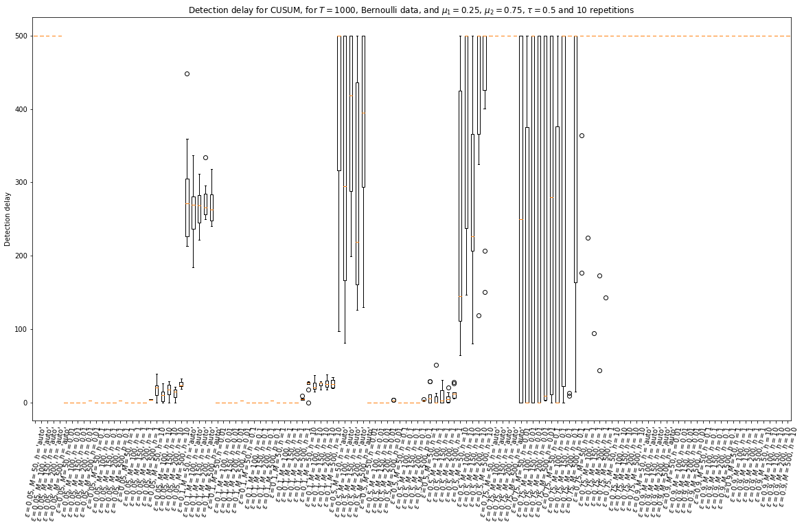
CPU times: user 54.2 s, sys: 1.89 s, total: 56.1 s
Wall time: 3min 48s
Now for the first problem (\(T=1000\)) and the PHT algorithm.
[306]:
%%time
_ = view1D_explore_parameters(detection_delay, "Detection delay",
PHT,
tau=tau,
firstMean=mu_1,
secondMean=mu_2,
horizon=horizon,
repetitions=10,
gaussian=False,
list_of_args_kwargs=list_of_args_kwargs_for_CUSUM,
argskwargs2str=argskwargs2str_for_CUSUM,
savefig=f"Detection_delay__PHT__Bernoulli_T1000_N10__params{len(list_of_args_kwargs_for_CUSUM)}",
)
Exploring detection_delay for algorithm <class '__main__.PHT'>, mu^1 = 0.25, mu^2 = 0.75, and horizon = 1000, tau = 500...
with 125 values for args, kwargs, and 10 repetitions.
Saving figure with format png, to file 'Detection_delay__PHT__Bernoulli_T1000_N10__params125.png'...
Saved! 'Detection_delay__PHT__Bernoulli_T1000_N10__params125.png' created of size '60939b', at 'Tue Dec 18 12:50:44 2018' ...
Saving figure with format pdf, to file 'Detection_delay__PHT__Bernoulli_T1000_N10__params125.pdf'...
Saved! 'Detection_delay__PHT__Bernoulli_T1000_N10__params125.pdf' created of size '31478b', at 'Tue Dec 18 12:50:54 2018' ...
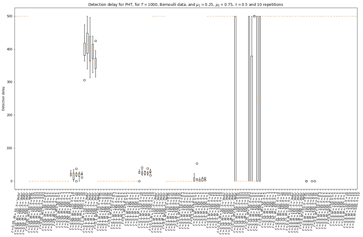
CPU times: user 51.8 s, sys: 1.8 s, total: 53.6 s
Wall time: 5min 24s
Then, for a Gaussian problem with the same gap:
[307]:
horizon = 1000
firstMean = mu_1 = -0.25
secondMean = mu_2 = 0.25
gap = mu_2 - mu_1
tau = 0.5
[308]:
%%time
_ = view1D_explore_parameters(detection_delay, "Detection delay",
CUSUM,
tau=tau,
firstMean=mu_1,
secondMean=mu_2,
horizon=horizon,
repetitions=10,
gaussian=True,
list_of_args_kwargs=list_of_args_kwargs_for_CUSUM,
argskwargs2str=argskwargs2str_for_CUSUM,
savefig=f"Detection_delay__CUSUM__Gaussian_T1000_N10__params{len(list_of_args_kwargs_for_CUSUM)}",
)
Exploring detection_delay for algorithm <class '__main__.CUSUM'>, mu^1 = -0.25, mu^2 = 0.25, and horizon = 1000, tau = 500...
with 125 values for args, kwargs, and 10 repetitions.
Saving figure with format png, to file 'Detection_delay__CUSUM__Gaussian_T1000_N10__params125.png'...
Saved! 'Detection_delay__CUSUM__Gaussian_T1000_N10__params125.png' created of size '64997b', at 'Tue Dec 18 12:53:39 2018' ...
Saving figure with format pdf, to file 'Detection_delay__CUSUM__Gaussian_T1000_N10__params125.pdf'...
Saved! 'Detection_delay__CUSUM__Gaussian_T1000_N10__params125.pdf' created of size '37037b', at 'Tue Dec 18 12:53:49 2018' ...
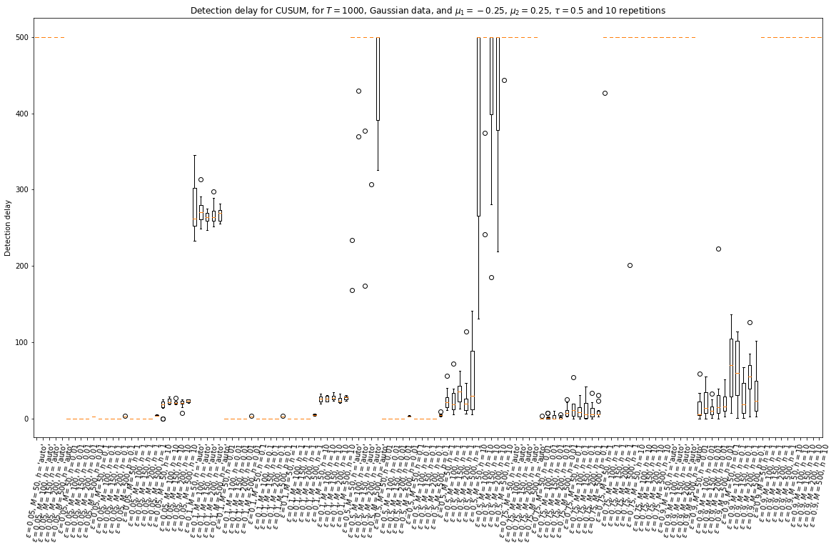
CPU times: user 50.9 s, sys: 1.46 s, total: 52.4 s
Wall time: 2min 54s
Experiments for Sub-Gaussian GLR
[293]:
list_of_args_kwargs_for_SubGaussianGLR = tuple([
((), {'delta': delta, 'joint': joint, 'sigma': sigma}) # empty args, kwargs = {delta=0.01, joint=True}
for joint in [True, False]
for delta in [10, 1, 0.1, 0.05, 0.01, 0.005, 0.001, 0.0005, 0.0001]
for sigma in [10*SIGMA, SIGMA, 0.1*SIGMA]
])
[294]:
def argskwargs2str_for_SubGaussianGLR(args, kwargs):
delta = kwargs['delta']
joint = kwargs['joint']
sigma = kwargs['sigma']
return fr"$\delta={delta:.4g}$, {'joint' if joint else 'disjoint'}, $\sigma={sigma:.4g}$"
First, for a Bernoulli problem:
[309]:
horizon = 1000
firstMean = mu_1 = 0.25
secondMean = mu_2 = 0.75
gap = mu_2 - mu_1
tau = 0.5
[310]:
%%time
_ = view1D_explore_parameters(detection_delay, "Detection delay",
SubGaussianGLR,
tau=tau,
firstMean=mu_1,
secondMean=mu_2,
horizon=horizon,
repetitions=10,
gaussian=False,
list_of_args_kwargs=list_of_args_kwargs_for_SubGaussianGLR,
argskwargs2str=argskwargs2str_for_SubGaussianGLR,
savefig=f"Detection_delay__SubGaussianGLR__Bernoulli_T1000_N10__params{len(list_of_args_kwargs_for_SubGaussianGLR)}",
)
Exploring detection_delay for algorithm <class '__main__.SubGaussianGLR'>, mu^1 = 0.25, mu^2 = 0.75, and horizon = 1000, tau = 500...
with 54 values for args, kwargs, and 10 repetitions.
Saving figure with format png, to file 'Detection_delay__SubGaussianGLR__Bernoulli_T1000_N10__params54.png'...
Saved! 'Detection_delay__SubGaussianGLR__Bernoulli_T1000_N10__params54.png' created of size '91097b', at 'Mon Dec 17 20:11:52 2018' ...
Saving figure with format pdf, to file 'Detection_delay__SubGaussianGLR__Bernoulli_T1000_N10__params54.pdf'...
Saved! 'Detection_delay__SubGaussianGLR__Bernoulli_T1000_N10__params54.pdf' created of size '23648b', at 'Tue Dec 18 12:56:29 2018' ...
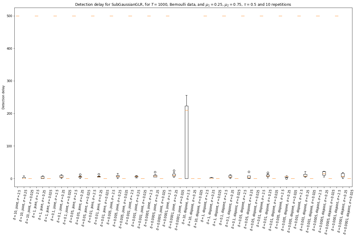
CPU times: user 19.9 s, sys: 1.13 s, total: 21.1 s
Wall time: 2min 25s
[311]:
%%time
_ = view1D_explore_parameters(false_alarm, "False alarm probability",
SubGaussianGLR,
tau=tau,
firstMean=mu_1,
secondMean=mu_2,
horizon=horizon,
repetitions=10,
gaussian=False,
list_of_args_kwargs=list_of_args_kwargs_for_SubGaussianGLR,
argskwargs2str=argskwargs2str_for_SubGaussianGLR,
savefig=f"False_alarm__SubGaussianGLR__Bernoulli_T1000_N10__params{len(list_of_args_kwargs_for_SubGaussianGLR)}",
)
Exploring false_alarm for algorithm <class '__main__.SubGaussianGLR'>, mu^1 = 0.25, mu^2 = 0.75, and horizon = 1000, tau = 500...
with 54 values for args, kwargs, and 10 repetitions.
Saving figure with format png, to file 'False_alarm__SubGaussianGLR__Bernoulli_T1000_N10__params54.png'...
Saved! 'False_alarm__SubGaussianGLR__Bernoulli_T1000_N10__params54.png' created of size '90523b', at 'Mon Dec 17 20:12:36 2018' ...
Saving figure with format pdf, to file 'False_alarm__SubGaussianGLR__Bernoulli_T1000_N10__params54.pdf'...
Saved! 'False_alarm__SubGaussianGLR__Bernoulli_T1000_N10__params54.pdf' created of size '23930b', at 'Tue Dec 18 12:57:51 2018' ...
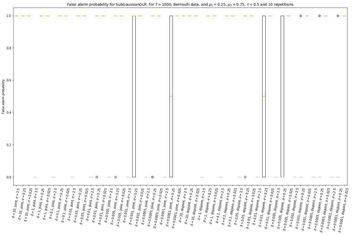
CPU times: user 20.3 s, sys: 1.13 s, total: 21.4 s
Wall time: 1min 20s
Then, for a Gaussian problem:
[314]:
horizon = 1000
firstMean = mu_1 = -0.1
secondMean = mu_2 = 0.1
gap = mu_2 - mu_1
tau = 0.5
[315]:
%%time
_ = view1D_explore_parameters(detection_delay, "Detection delay",
SubGaussianGLR,
tau=tau,
firstMean=mu_1,
secondMean=mu_2,
horizon=horizon,
repetitions=10,
gaussian=True,
list_of_args_kwargs=list_of_args_kwargs_for_SubGaussianGLR,
argskwargs2str=argskwargs2str_for_SubGaussianGLR,
savefig=f"Detection_delay__SubGaussianGLR__Gaussian_T1000_N10__params{len(list_of_args_kwargs_for_SubGaussianGLR)}",
)
Exploring detection_delay for algorithm <class '__main__.SubGaussianGLR'>, mu^1 = -0.1, mu^2 = 0.1, and horizon = 1000, tau = 500...
with 54 values for args, kwargs, and 10 repetitions.
Saving figure with format png, to file 'Detection_delay__SubGaussianGLR__Gaussian_T1000_N10__params54.png'...
Saved! 'Detection_delay__SubGaussianGLR__Gaussian_T1000_N10__params54.png' created of size '91989b', at 'Mon Dec 17 20:13:24 2018' ...
Saving figure with format pdf, to file 'Detection_delay__SubGaussianGLR__Gaussian_T1000_N10__params54.pdf'...
Saved! 'Detection_delay__SubGaussianGLR__Gaussian_T1000_N10__params54.pdf' created of size '24191b', at 'Tue Dec 18 13:11:55 2018' ...
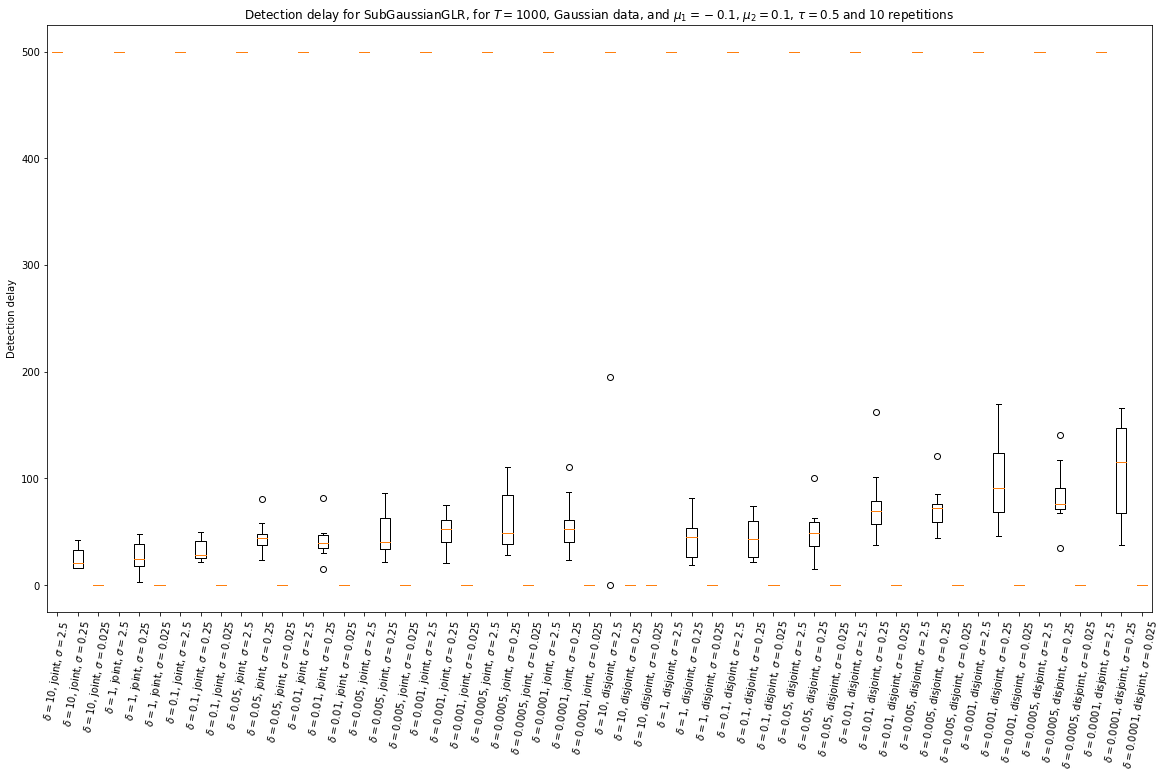
CPU times: user 23.8 s, sys: 1.34 s, total: 25.1 s
Wall time: 3min 2s
And for a harder Gaussian problem:
[312]:
horizon = 1000
firstMean = mu_1 = -0.01
secondMean = mu_2 = 0.01
gap = mu_2 - mu_1
tau = 0.5
[313]:
%%time
_ = view1D_explore_parameters(detection_delay, "Detection delay",
SubGaussianGLR,
tau=tau,
firstMean=mu_1,
secondMean=mu_2,
horizon=horizon,
repetitions=10,
gaussian=True,
list_of_args_kwargs=list_of_args_kwargs_for_SubGaussianGLR,
argskwargs2str=argskwargs2str_for_SubGaussianGLR,
savefig=f"Detection_delay__SubGaussianGLR__Gaussian_T1000_N10__params{len(list_of_args_kwargs_for_SubGaussianGLR)}_2",
)
Exploring detection_delay for algorithm <class '__main__.SubGaussianGLR'>, mu^1 = -0.01, mu^2 = 0.01, and horizon = 1000, tau = 500...
with 54 values for args, kwargs, and 10 repetitions.
Saving figure with format png, to file 'Detection_delay__SubGaussianGLR__Gaussian_T1000_N10__params54_2.png'...
Saved! 'Detection_delay__SubGaussianGLR__Gaussian_T1000_N10__params54_2.png' created of size '89392b', at 'Mon Dec 17 20:14:23 2018' ...
Saving figure with format pdf, to file 'Detection_delay__SubGaussianGLR__Gaussian_T1000_N10__params54_2.pdf'...
Saved! 'Detection_delay__SubGaussianGLR__Gaussian_T1000_N10__params54_2.pdf' created of size '21779b', at 'Tue Dec 18 13:02:19 2018' ...
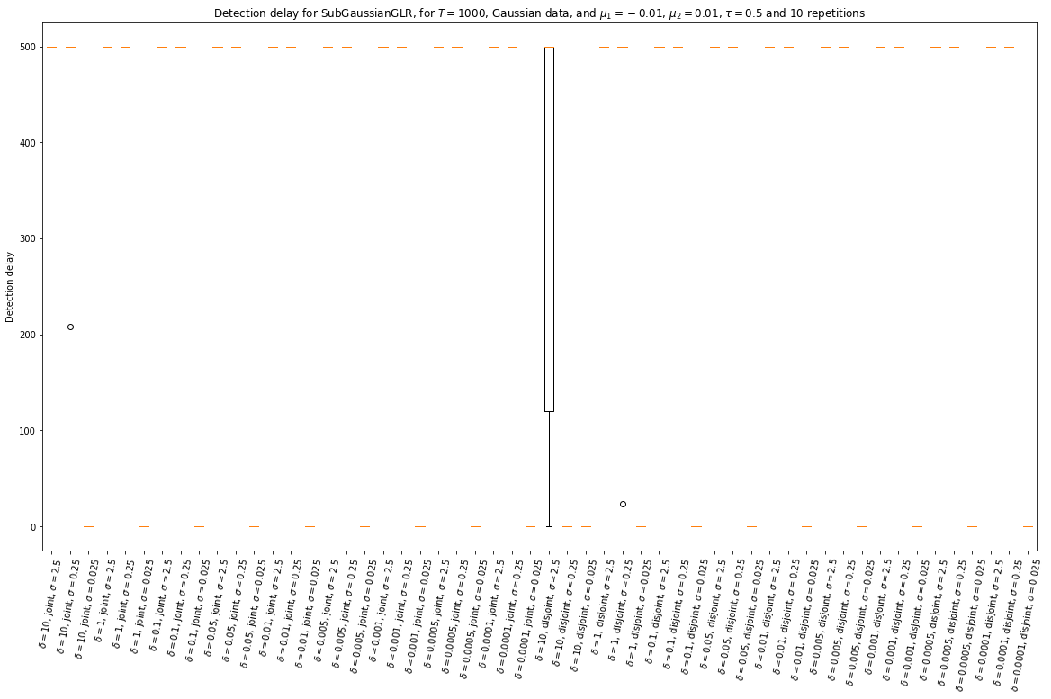
CPU times: user 21.9 s, sys: 1.12 s, total: 23 s
Wall time: 4min 29s
Other experiments
[ ]:
Conclusions
TODO TODO TODO TODO TODO TODO